MODULE 13 · Progressive training: understand, calculate, verify.

Living and working elsewhere: from landing site to society

Premium growth-thresholds diagram for a Mars settlement, from outpost to city. — A settlement changes architecture as it grows — teaching summary diagram for this module.

Living elsewhere connects site, energy, water, transport, construction, maintenance, industry, health, and skills. Every choice opens and closes options.

This module assembles earlier tools and compares architectures at 4, 20, 100, and 1,000 inhabitants without prescribing one Mars city.

1. Choose a site: science, resources, operations

NASA used the Exploration Zone concept: regions of interest roughly within 100 km of a central landing site so science, resources, and operations could be considered together. The radius is a historical study framework, not a universal settlement rule.

Site choice combines altitude for EDL, slope, rocks, accessible ice or minerals, energy, dust, communications, geologic hazards, and science value. An excellent resource in a cargo-hostile location can be less useful than a modest resource inside a robust architecture.

Site study — turn a radius into an operations problem

NASA’s historical Exploration Zone concept grouped regions of interest within roughly 100 km of a central landing site. A 100 km-radius circle has geometric area πr² ≈ 31,400 km², but that area is obviously not all usable: slopes, rocks, terrain hazards, and scientific targets fragment it. The calculation only exposes the spatial scale of the mobility problem.

A round trip to a point 80 km from the centre is at least 160 km of ideal travel before detours. At a teaching average operational speed of 10 km/h, that is 16 hours of driving alone. Add sampling, stops, charging, weather, and rescue margin and “a resource 80 km away” becomes a mission rather than a dot on a map. Site selection must therefore connect resource value to actual reachability.

Search area and mobility distance

A = π r²

1 — Concrete question: What operational question does this relation answer for search area and mobility distance?
2 — Intuition without symbols: A radius defines a circular search area, while each destination also imposes a real round-trip distance.
3 — Quantities first: A is area and r search radius.
4 — Formula: A = π r²
5 — Read aloud: Read the relation aloud term by term: A = π r².
6 — Symbols and meaning: A is area and r search radius.
7 — Pronunciation: The “Read aloud” line above is the oral reference for “Search area and mobility distance”. Any subscript, exponent or grouping that changes the meaning of the relation should be spoken explicitly.
8 — Units: If r is in kilometres, A is in square kilometres.
9 — Convention: For “Search area and mobility distance”, substitute values without changing the reference frame, time basis, system boundary or sign convention halfway through the calculation. Stated units: If r is in kilometres, A is in square kilometres.
10 — Why this operation: A radius defines a circular search area, while each destination also imposes a real round-trip distance.
11 — Assumptions: The relation “A = π r²” applies here only to the scenario described by the card. Inputs must be mutually consistent and satisfy the physical assumptions associated with “Search area and mobility distance”.
12 — Unit check: If r is in kilometres, A is in square kilometres. Verify that units reduce to the unit of the requested quantity.
13 — Numerical case: Teaching example: for r = 100 km, A = π × 100² ≈ 31,416 km². A destination 80 km away already implies a 160 km ideal round trip.
14 — Why the calculation works: A radius defines a circular search area, while each destination also imposes a real round-trip distance.
15 — Algebra check: Quick check: invert “A = π r²” when possible, or use a second calculation path, and confirm the same order of magnitude for “Search area and mobility distance”.
16 — Mental estimate: Before calculating “Search area and mobility distance” precisely, round the inputs to one useful digit and predict the sign and order of magnitude. The detailed result should remain consistent with that estimate.
17 — Interpretation: The result is useful only as an operational statement about search area and mobility distance under the declared assumptions.
18 — What the result does not prove: For “Search area and mobility distance”, the number obtained answers only the model “A = π r²” under the stated scenario. It does not by itself validate the input data or the model outside those conditions.
19 — Sensitivity: Vary one input at a time around the nominal case to identify what drives the result of “Search area and mobility distance” and whether that variation can change the mission decision.
20 — Guided and autonomous practice: Guided exercise. Increase search radius by 10%, from 100 to 110 km. Recompute accessible area and compare with the initial case.
Detailed guided correction — open after attempting
Detailed correction. A = π × 110² = π × 12,100 ≈ 38,013 km². Radius rises by 10%, but area follows the square: 38,013/31,416 ≈ 1.21, or about +21%. Logistics therefore grows faster than linear distance.
Autonomous exercise. Build a second numerical scenario for “Search area and mobility distance” by changing at least two inputs in A = π r². Compute the result, check units and order of magnitude, then state whether the mission decision should change.
Autonomous correction — specific criteria
Autonomous correction. The answer must show substitution into A = π r², produce a value with its unit or an explicit logical result, compare it with the reference case, and justify the following decision: Never confuse a large theoretical area with real operational terrain accessibility.
21 — Mission decision: Never confuse a large theoretical area with real operational terrain accessibility.

System intuition

Choosing a site solves several problems at once: landing safety, water access, energy, science, traversable terrain, communications, and room to expand. NASA’s Exploration Zone concept places several regions of interest within roughly 100 km, but that geometry does not guarantee operational access.

Multi-criteria site score

S_site = Σ w_i s_i

1 — Concrete question: What operational question does this relation answer for multi-criteria site score?
2 — Intuition without symbols: Each site criterion counts according to its importance, then weighted contributions are summed to compare options on a common basis.
3 — Quantities first: w_i is the weight of criterion i, s_i its score, and S_site the total weighted score.
4 — Formula: S_site = Σ w_i s_i
5 — Read aloud: Read the relation aloud term by term: S_site = Σ w_i s_i.
6 — Symbols and meaning: w_i is the weight of criterion i, s_i its score, and S_site the total weighted score.
7 — Pronunciation: The “Read aloud” line above is the oral reference for “Multi-criteria site score”. Any subscript, exponent or grouping that changes the meaning of the relation should be spoken explicitly.
8 — Units: Weights are dimensionless and normally sum to one; criterion scores use one common scale.
9 — Convention: For “Multi-criteria site score”, substitute values without changing the reference frame, time basis, system boundary or sign convention halfway through the calculation. Stated units: Weights are dimensionless and normally sum to one; criterion scores use one common scale.
10 — Why this operation: Each site criterion counts according to its importance, then weighted contributions are summed to compare options on a common basis.
11 — Assumptions: The relation “S_site = Σ w_i s_i” applies here only to the scenario described by the card. Inputs must be mutually consistent and satisfy the physical assumptions associated with “Multi-criteria site score”.
12 — Unit check: Weights are dimensionless and normally sum to one; criterion scores use one common scale. Verify that units reduce to the unit of the requested quantity.
13 — Numerical case: Teaching example: with weights 0.30, 0.20, 0.15, 0.15, 0.10, 0.10 and scores 8, 9, 7, 8, 6, 6.5, S_site = 7.70.
14 — Why the calculation works: Each site criterion counts according to its importance, then weighted contributions are summed to compare options on a common basis.
15 — Algebra check: Quick check: invert “S_site = Σ w_i s_i” when possible, or use a second calculation path, and confirm the same order of magnitude for “Multi-criteria site score”.
16 — Mental estimate: Before calculating “Multi-criteria site score” precisely, round the inputs to one useful digit and predict the sign and order of magnitude. The detailed result should remain consistent with that estimate.
17 — Interpretation: The result is useful only as an operational statement about multi-criteria site score under the declared assumptions.
18 — What the result does not prove: For “Multi-criteria site score”, the number obtained answers only the model “S_site = Σ w_i s_i” under the stated scenario. It does not by itself validate the input data or the model outside those conditions.
19 — Sensitivity: Vary one input at a time around the nominal case to identify what drives the result of “Multi-criteria site score” and whether that variation can change the mission decision.
20 — Guided and autonomous practice: Guided exercise. Increase the first score by 10%, from 8 to 8.8, with weights and other scores unchanged. Recompute S_site.
Detailed guided correction — open after attempting
Detailed correction. The first contribution rises from 0.30×8 = 2.40 to 0.30×8.8 = 2.64, a +0.24 change. Total score therefore rises from 7.70 to 7.94. The 0.30 weight limits the effect of a local improvement on the total score.
Autonomous exercise. Build a second numerical scenario for “Multi-criteria site score” by changing at least two inputs in S_site = Σ w_i s_i. Compute the result, check units and order of magnitude, then state whether the mission decision should change.
Autonomous correction — specific criteria
Autonomous correction. The answer must show substitution into S_site = Σ w_i s_i, produce a value with its unit or an explicit logical result, compare it with the reference case, and justify the following decision: Use the score to expose trade-offs while keeping safety veto criteria separate.
21 — Mission decision: Use the score to expose trade-offs while keeping safety veto criteria separate.

Criterion weights change the decision; a score is useful only when its assumptions are explicit.

Site case — multiple criteria

Compare two sites: A has closer water but harder terrain; B requires 20 km more travel to water but offers easier landing and routes. A trade matrix should translate each advantage into measurable consequences—transport mass, EVA time, energy, failure frequency, and rescue access—rather than adjectives such as “better” or “promising.”

2. Predeploy before crew

Sending power, communications, inventory, and perhaps local production before people converts time into evidence. Equipment can accumulate operating hours and reveal faults before crew commitment.

Predeployed cargo can fail, land far away, or age in place. A robust campaign identifies what must work before departure, what requires duplication, and which failure combinations cancel a crew mission.

Quantified balance

Predeployment reduces human risk only when systems can be remotely tested in representative states. Cargo that has landed but cannot be connected, calibrated, or repaired is not an available capability. Cargo campaigns therefore need activation sequences, telemetry, spares, and acceptance criteria.

Actually ready capacity

ready_capacity = delivered × activated × validated

1 — Concrete question: What operational question does this relation answer for actually ready capacity?
2 — Intuition without symbols: Delivered capability is not yet available: it must be activated and validated before the mission can credit it.
3 — Quantities first: Delivered, activated and validated are fractions or stage efficiencies applied to nominal capability.
4 — Formula: ready_capacity = delivered × activated × validated
5 — Read aloud: Read the relation aloud term by term: ready_capacity = delivered × activated × validated.
6 — Symbols and meaning: Delivered, activated and validated are fractions or stage efficiencies applied to nominal capability.
7 — Pronunciation: The “Read aloud” line above is the oral reference for “Actually ready capacity”. Any subscript, exponent or grouping that changes the meaning of the relation should be spoken explicitly.
8 — Units: A capability unit multiplied by dimensionless fractions remains in the same capability unit.
9 — Convention: For “Actually ready capacity”, substitute values without changing the reference frame, time basis, system boundary or sign convention halfway through the calculation. Stated units: A capability unit multiplied by dimensionless fractions remains in the same capability unit.
10 — Why this operation: Delivered capability is not yet available: it must be activated and validated before the mission can credit it.
11 — Assumptions: The relation “ready_capacity = delivered × activated × validated” applies here only to the scenario described by the card. Inputs must be mutually consistent and satisfy the physical assumptions associated with “Actually ready capacity”.
12 — Unit check: A capability unit multiplied by dimensionless fractions remains in the same capability unit. Verify that units reduce to the unit of the requested quantity.
13 — Numerical case: Teaching example: 100 delivered units, 90% activated, and 95% validated gives ready_capacity = 100 × 0.90 × 0.95 = 85.5 units.
14 — Why the calculation works: Delivered capability is not yet available: it must be activated and validated before the mission can credit it.
15 — Algebra check: Quick check: for any non-zero factor, dividing the result by that factor should recover the other expected contribution in “Actually ready capacity”.
16 — Mental estimate: Before calculating “Actually ready capacity” precisely, round the inputs to one useful digit and predict the sign and order of magnitude. The detailed result should remain consistent with that estimate.
17 — Interpretation: The result is useful only as an operational statement about actually ready capacity under the declared assumptions.
18 — What the result does not prove: For “Actually ready capacity”, the number obtained answers only the model “ready_capacity = delivered × activated × validated” under the stated scenario. It does not by itself validate the input data or the model outside those conditions.
19 — Sensitivity: Vary one input at a time around the nominal case to identify what drives the result of “Actually ready capacity” and whether that variation can change the mission decision.
20 — Guided and autonomous practice: Guided exercise. Increase delivered capacity by 10%, from 100 to 110 units, keeping activation and validation unchanged. Recompute ready capacity.
Detailed guided correction — open after attempting
Detailed correction. ready_capacity = 110 × 0.90 × 0.95 = 94.05 units. The combined fractions remain 0.855, so +10% delivered capacity gives +10% actually ready capacity, from 85.5 to 94.05 units.
Autonomous exercise. Build a second numerical scenario for “Actually ready capacity” by changing at least two inputs in ready_capacity = delivered × activated × validated. Compute the result, check units and order of magnitude, then state whether the mission decision should change.
Autonomous correction — specific criteria
Autonomous correction. The answer must show substitution into ready_capacity = delivered × activated × validated, produce a value with its unit or an explicit logical result, compare it with the reference case, and justify the following decision: Do not grow crew size based on capability that has not yet been validated.
21 — Mission decision: Do not grow crew size based on capability that has not yet been validated.

Adding flights does not automatically multiply reliability when they share a common design defect.

Cargo case — real availability

A water plant is predeployed in two modules. Both land, but a water-quality sensor fails and no backup standard is available. The mass is on Mars, yet the capability “qualified water” has not been demonstrated. Remote acceptance must test the end function, not merely electrical presence of hardware.

Decision check. Predeployment should include a formal readiness matrix: landed, powered, communicating, calibrated, functionally tested, stocked, and recoverable. A check mark under “landed” is only the first state. The crew should leave Earth only after the campaign has demonstrated the set of functions that must already exist on Mars.

3. Energy: infrastructure beneath all other infrastructure

Pumping, heating, compressing, lighting, recycling, manufacturing, and communication consume power. Budgets must separate average load, peaks, storage, availability, and critical loads. Installed power is not the same as available power during a fault.

NASA still describes the Mars Architecture Trade Space in March 2026 as relatively open. Some choices narrow the options, while transport and surface architecture remain evolvable. A Mars study should preserve technology status rather than treat a concept as accomplished capability.

Premium poster of a permanent Mars settlement linking habitat, life support, transport, industry, people and governance. — Choosing a site is only the beginning: a permanent settlement must connect transport, habitat, life support, people, industry and governance.

Degraded mode

Energy connects every function to a time constraint. An industrial plant may draw much power yet tolerate interruption; ECLSS may draw less but require near-continuous service. Loads must therefore be ranked by criticality with shedding, restart, and black-start plans.

Critical energy reserve

E_reserve = P_critical × t_without_generation

1 — Concrete question: What operational question does this relation answer for critical energy reserve?
2 — Intuition without symbols: A critical load needs enough stored energy to bridge the whole period during which reliable generation is unavailable.
3 — Quantities first: P_critical is protected power and t_without_generation the protected outage duration.
4 — Formula: E_reserve = P_critical × t_without_generation
5 — Read aloud: Read the relation aloud term by term: E_reserve = P_critical × t_without_generation.
6 — Symbols and meaning: P_critical is protected power and t_without_generation the protected outage duration.
7 — Pronunciation: The “Read aloud” line above is the oral reference for “Critical energy reserve”. Any subscript, exponent or grouping that changes the meaning of the relation should be spoken explicitly.
8 — Units: kW multiplied by h gives kWh.
9 — Convention: For “Critical energy reserve”, substitute values without changing the reference frame, time basis, system boundary or sign convention halfway through the calculation. Stated units: kW multiplied by h gives kWh.
10 — Why this operation: A critical load needs enough stored energy to bridge the whole period during which reliable generation is unavailable.
11 — Assumptions: The relation “E_reserve = P_critical × t_without_generation” applies here only to the scenario described by the card. Inputs must be mutually consistent and satisfy the physical assumptions associated with “Critical energy reserve”.
12 — Unit check: kW multiplied by h gives kWh. Verify that units reduce to the unit of the requested quantity.
13 — Numerical case: Teaching example: a critical load P_critical = 5 kW protected for t_without_generation = 12 h requires E_reserve = 5 × 12 = 60 kWh before losses and margin.
14 — Why the calculation works: A critical load needs enough stored energy to bridge the whole period during which reliable generation is unavailable.
15 — Algebra check: Quick check: for any non-zero factor, dividing the result by that factor should recover the other expected contribution in “Critical energy reserve”.
16 — Mental estimate: Before calculating “Critical energy reserve” precisely, round the inputs to one useful digit and predict the sign and order of magnitude. The detailed result should remain consistent with that estimate.
17 — Interpretation: The result is useful only as an operational statement about critical energy reserve under the declared assumptions.
18 — What the result does not prove: For “Critical energy reserve”, the number obtained answers only the model “E_reserve = P_critical × t_without_generation” under the stated scenario. It does not by itself validate the input data or the model outside those conditions.
19 — Sensitivity: Vary one input at a time around the nominal case to identify what drives the result of “Critical energy reserve” and whether that variation can change the mission decision.
20 — Guided and autonomous practice: Guided exercise. Increase no-generation duration by 10%, from 12 to 13.2 h, keeping 5 kW. Recompute minimum reserve.
Detailed guided correction — open after attempting
Detailed correction. E_reserve = 5 × 13.2 = 66 kWh. Duration enters linearly, so +10% duration requires +10% minimum energy, or +6 kWh above the initial 60 kWh before losses and margin.
Autonomous exercise. Build a second numerical scenario for “Critical energy reserve” by changing at least two inputs in E_reserve = P_critical × t_without_generation. Compute the result, check units and order of magnitude, then state whether the mission decision should change.
Autonomous correction — specific criteria
Autonomous correction. The answer must show substitution into E_reserve = P_critical × t_without_generation, produce a value with its unit or an explicit logical result, compare it with the reference case, and justify the following decision: Size reserve from the real critical load and a credible loss-of-generation scenario.
21 — Mission decision: Size reserve from the real critical load and a credible loss-of-generation scenario.

Storage must support peak power and startup current, not merely total energy.

Energy case — black start

After a total outage, critical loads total 35 kW but pumps and compressors need a 60 kW startup peak for 20 s. A battery with 100 kWh energy but only 45 kW power cannot restart the system without sequencing or another source. Stored energy and black-start power are separate constraints.

4. Water, air, food: shift from inventory to flow

Early missions can be dominated by imported stock. As duration and population grow, flows dominate. Ten tonnes sounds large until a 400 kg/day net loss consumes it in 25 days.

Recycling reduces imports while adding filters, sensors, power, and maintenance. Crops can reduce some food imports but demand water, nutrients, light, and sanitation. Autonomy is a network of coupled flows.

Safety reading

Water, air, and food move from inventory to flow as population and duration increase. The useful metric becomes daily deficit after recycling and local production. Large stocks remain valuable for failures but cannot indefinitely hide a structurally deficient loop.

Inventory change

Delta stock = production + import − consumption − losses

1 — Concrete question: What operational question does this relation answer for inventory change?
2 — Intuition without symbols: Final inventory depends on every flow crossing the same system boundary during the same period.
3 — Quantities first: Production and imports add inventory; consumption and losses remove it.
4 — Formula: Delta stock = production + import − consumption − losses
5 — Read aloud: Read the relation aloud term by term: Delta stock = production + import − consumption − losses.
6 — Symbols and meaning: Production and imports add inventory; consumption and losses remove it.
7 — Pronunciation: The “Read aloud” line above is the oral reference for “Inventory change”. Any subscript, exponent or grouping that changes the meaning of the relation should be spoken explicitly.
8 — Units: All terms use the same resource unit over the same accounting period.
9 — Convention: For “Inventory change”, substitute values without changing the reference frame, time basis, system boundary or sign convention halfway through the calculation. Stated units: All terms use the same resource unit over the same accounting period.
10 — Why this operation: Final inventory depends on every flow crossing the same system boundary during the same period.
11 — Assumptions: The relation “Delta stock = production + import − consumption − losses” applies here only to the scenario described by the card. Inputs must be mutually consistent and satisfy the physical assumptions associated with “Inventory change”.
12 — Unit check: All terms use the same resource unit over the same accounting period. Verify that units reduce to the unit of the requested quantity.
13 — Numerical case: Teaching example: production 10 units + import 2 − consumption 8 − losses 2 gives Δstock = +2 units over the period.
14 — Why the calculation works: Final inventory depends on every flow crossing the same system boundary during the same period.
15 — Algebra check: Quick check: adding the subtracted term back to the result should reconstruct the starting quantity in “Inventory change”.
16 — Mental estimate: Before calculating “Inventory change” precisely, round the inputs to one useful digit and predict the sign and order of magnitude. The detailed result should remain consistent with that estimate.
17 — Interpretation: The result is useful only as an operational statement about inventory change under the declared assumptions.
18 — What the result does not prove: For “Inventory change”, the number obtained answers only the model “Delta stock = production + import − consumption − losses” under the stated scenario. It does not by itself validate the input data or the model outside those conditions.
19 — Sensitivity: Vary one input at a time around the nominal case to identify what drives the result of “Inventory change” and whether that variation can change the mission decision.
20 — Guided and autonomous practice: Guided exercise. Increase consumption by 10%, from 8 to 8.8 units, with all other terms unchanged. Recompute Δstock.
Detailed guided correction — open after attempting
Detailed correction. Δstock = 10 + 2 − 8.8 − 2 = +1.2 units. Inventory still grows, but net margin falls from +2 to +1.2: 0.8 unit of margin has been consumed.
Autonomous exercise. Build a second numerical scenario for “Inventory change” by changing at least two inputs in Delta stock = production + import − consumption − losses. Compute the result, check units and order of magnitude, then state whether the mission decision should change.
Autonomous correction — specific criteria
Autonomous correction. The answer must show substitution into Delta stock = production + import − consumption − losses, produce a value with its unit or an explicit logical result, compare it with the reference case, and justify the following decision: Expose any negative trend before it becomes a stockout.
21 — Mission decision: Expose any negative trend before it becomes a stockout.

A loop stable on average can still face demand peaks; buffers size timing mismatches, not just annual balance.

Flow case — buffer

An oxygen plant averages 45 kg/day while demand averages 40 kg/day. During five maintenance days production falls to zero. The nominal 5 kg/day surplus does not describe safety: at least 200 kg is needed to cover maintenance, plus margin, before the daily surplus can rebuild inventory.

Decision check. Flow thinking also changes how margins are reported. Instead of saying “we have 100 tonnes of water,” operations should know days of reserve at nominal demand, days at emergency demand, local production rate, repair time, and the rate at which the reserve can be rebuilt after an outage.

5. Local construction: think in tonnes

Teaching case: 2 m regolith cover, assumed bulk density 1,500 kg/m³, over 100 m². Moved mass = 2 × 1,500 × 100 = 300,000 kg = 300 t.

Shielding mass

M = e rho A

1 — Concrete question: What operational question does this relation answer for shielding mass?
2 — Intuition without symbols: Thickness over an area gives material volume, and density converts that volume into logistics mass.
3 — Quantities first: e is thickness, rho density, A covered area, and M shielding mass.
4 — Formula: M = e rho A
5 — Read aloud: Read the relation aloud term by term: M = e rho A.
6 — Symbols and meaning: e is thickness, rho density, A covered area, and M shielding mass.
7 — Pronunciation: The “Read aloud” line above is the oral reference for “Shielding mass”. Any subscript, exponent or grouping that changes the meaning of the relation should be spoken explicitly.
8 — Units: m × kg/m³ × m² gives kg.
9 — Convention: For “Shielding mass”, substitute values without changing the reference frame, time basis, system boundary or sign convention halfway through the calculation. Stated units: m × kg/m³ × m² gives kg.
10 — Why this operation: Thickness over an area gives material volume, and density converts that volume into logistics mass.
11 — Assumptions: The relation “M = e rho A” applies here only to the scenario described by the card. Inputs must be mutually consistent and satisfy the physical assumptions associated with “Shielding mass”.
12 — Unit check: m × kg/m³ × m² gives kg. Verify that units reduce to the unit of the requested quantity.
13 — Numerical case: Teaching example: e = 2 m, ρ = 1,500 kg/m³, and A = 100 m² gives M = 2 × 1,500 × 100 = 300,000 kg, or 300 t.
14 — Why the calculation works: Thickness over an area gives material volume, and density converts that volume into logistics mass.
15 — Algebra check: Quick check: invert “M = e rho A” when possible, or use a second calculation path, and confirm the same order of magnitude for “Shielding mass”.
16 — Mental estimate: Before calculating “Shielding mass” precisely, round the inputs to one useful digit and predict the sign and order of magnitude. The detailed result should remain consistent with that estimate.
17 — Interpretation: The result is useful only as an operational statement about shielding mass under the declared assumptions.
18 — What the result does not prove: For “Shielding mass”, the number obtained answers only the model “M = e rho A” under the stated scenario. It does not by itself validate the input data or the model outside those conditions.
19 — Sensitivity: Vary one input at a time around the nominal case to identify what drives the result of “Shielding mass” and whether that variation can change the mission decision.
20 — Guided and autonomous practice: Guided exercise. Increase thickness by 10%, from 2.0 to 2.2 m, keeping density and area unchanged. Recompute mass.
Detailed guided correction — open after attempting
Detailed correction. M = 2.2 × 1,500 × 100 = 330,000 kg = 330 t. A 10% thickness increase gives +10% mass at constant area and density: 30 t more to move.
Autonomous exercise. Build a second numerical scenario for “Shielding mass” by changing at least two inputs in M = e rho A. Compute the result, check units and order of magnitude, then state whether the mission decision should change.
Autonomous correction — specific criteria
Autonomous correction. The answer must show substitution into M = e rho A, produce a value with its unit or an explicit logical result, compare it with the reference case, and justify the following decision: Compare moved mass, energy, machine time, and radiation benefit before selecting a shielding architecture.
21 — Mission decision: Compare moved mass, energy, machine time, and radiation benefit before selecting a shielding architecture.

At average 250 kg/h, that is 1,200 h or 50 ideal continuous days. Charging, maintenance, relocation, weather, and quality control extend it. “Use regolith” becomes measurable industrial work.

Construction study — 300 tonnes of regolith is work, not a sketch

Take a teaching shielding layer 2 m thick, assumed bulk density 1,500 kg/m³, over 100 m². Moved mass is 2×1,500×100 = 300,000 kg or 300 t. A chain actually processing 250 kg/h requires 1,200 productive hours, equal to 50 ideal continuous days.

Calendar time is longer. At 70% availability, 1,200 productive hours require about 1,714 calendar hours or 71.4 days. If the machine averages 15 kW while working, productive energy is 18,000 kWh before charging and conversion losses. Local construction, power, maintenance, and logistics are therefore one architecture. Regolith is local; the work required to move it is not free.

Productive time and calendar time

t_productive = M / rate ; t_calendar = t_productive / availability

1 — Concrete question: What operational question does this relation answer for productive time and calendar time?
2 — Intuition without symbols: Useful operating time comes from required mass and real throughput; downtime then stretches the calendar duration.
3 — Quantities first: M is required mass, rate productive throughput, availability the productive fraction, and the two times are productive and calendar time.
4 — Formula: t_productive = M / rate ; t_calendar = t_productive / availability
5 — Read aloud: Read the relation aloud term by term: t_productive = M / rate ; t_calendar = t_productive / availability.
6 — Symbols and meaning: M is required mass, rate productive throughput, availability the productive fraction, and the two times are productive and calendar time.
7 — Pronunciation: The “Read aloud” line above is the oral reference for “Productive time and calendar time”. Any subscript, exponent or grouping that changes the meaning of the relation should be spoken explicitly.
8 — Units: Mass divided by mass/hour gives hours; dividing by dimensionless availability keeps hours.
9 — Convention: For “Productive time and calendar time”, substitute values without changing the reference frame, time basis, system boundary or sign convention halfway through the calculation. Stated units: Mass divided by mass/hour gives hours; dividing by dimensionless availability keeps hours.
10 — Why this operation: Useful operating time comes from required mass and real throughput; downtime then stretches the calendar duration.
11 — Assumptions: The relation “t_productive = M / rate ; t_calendar = t_productive / availability” applies here only to the scenario described by the card. Inputs must be mutually consistent and satisfy the physical assumptions associated with “Productive time and calendar time”.
12 — Unit check: Mass divided by mass/hour gives hours; dividing by dimensionless availability keeps hours. Verify that units reduce to the unit of the requested quantity.
13 — Numerical case: Teaching example: M = 300,000 kg and rate = 250 kg/h gives t_productive = 1,200 h. With availability 0.70, t_calendar = 1,200/0.70 ≈ 1,714 h.
14 — Why the calculation works: Useful operating time comes from required mass and real throughput; downtime then stretches the calendar duration.
15 — Algebra check: Quick check: multiplying the result by the denominator should reconstruct the numerator of “Productive time and calendar time” within rounding.
16 — Mental estimate: Before calculating “Productive time and calendar time” precisely, round the inputs to one useful digit and predict the sign and order of magnitude. The detailed result should remain consistent with that estimate.
17 — Interpretation: The result is useful only as an operational statement about productive time and calendar time under the declared assumptions.
18 — What the result does not prove: For “Productive time and calendar time”, the number obtained answers only the model “t_productive = M / rate ; t_calendar = t_productive / availability” under the stated scenario. It does not by itself validate the input data or the model outside those conditions.
19 — Sensitivity: Vary one input at a time around the nominal case to identify what drives the result of “Productive time and calendar time” and whether that variation can change the mission decision.
20 — Guided and autonomous practice: Guided exercise. Increase rate by 10%, from 250 to 275 kg/h, with M = 300,000 kg and availability = 0.70. Recompute both times.
Detailed guided correction — open after attempting
Detailed correction. t_productive = 300,000/275 = 1,090.9 h. t_calendar = 1,090.9/0.70 = 1,558.4 h. Calendar-time gain is 1,714.3 − 1,558.4 ≈ 155.9 h, about 6.5 days.
Autonomous exercise. Build a second numerical scenario for “Productive time and calendar time” by changing at least two inputs in t_productive = M / rate ; t_calendar = t_productive / availability. Compute the result, check units and order of magnitude, then state whether the mission decision should change.
Autonomous correction — specific criteria
Autonomous correction. The answer must show substitution into t_productive = M / rate ; t_calendar = t_productive / availability, produce a value with its unit or an explicit logical result, compare it with the reference case, and justify the following decision: Plan with calendar time rather than nominal operating time alone.
21 — Mission decision: Plan with calendar time rather than nominal operating time alone.

System intuition

Local construction should be expressed in tonnes, machine hours, and verified quality. Shielding thickness, area, and volume quickly become hundreds of tonnes, turning a material choice into excavation, transport, power, and maintenance.

Geometric material mass

M = A e rho

1 — Concrete question: What operational question does this relation answer for geometric material mass?
2 — Intuition without symbols: Area, thickness, and density turn a layer geometry directly into material mass.
3 — Quantities first: A is area, e thickness, rho density, and M mass.
4 — Formula: M = A e rho
5 — Read aloud: Read the relation aloud term by term: M = A e rho.
6 — Symbols and meaning: A is area, e thickness, rho density, and M mass.
7 — Pronunciation: The “Read aloud” line above is the oral reference for “Geometric material mass”. Any subscript, exponent or grouping that changes the meaning of the relation should be spoken explicitly.
8 — Units: m² × m × kg/m³ gives kg.
9 — Convention: For “Geometric material mass”, substitute values without changing the reference frame, time basis, system boundary or sign convention halfway through the calculation. Stated units: m² × m × kg/m³ gives kg.
10 — Why this operation: Area, thickness, and density turn a layer geometry directly into material mass.
11 — Assumptions: The relation “M = A e rho” applies here only to the scenario described by the card. Inputs must be mutually consistent and satisfy the physical assumptions associated with “Geometric material mass”.
12 — Unit check: m² × m × kg/m³ gives kg. Verify that units reduce to the unit of the requested quantity.
13 — Numerical case: Teaching example: A = 120 m², e = 0.50 m, and ρ = 2,000 kg/m³ gives M = 120 × 0.50 × 2,000 = 120,000 kg.
14 — Why the calculation works: Area, thickness, and density turn a layer geometry directly into material mass.
15 — Algebra check: Quick check: invert “M = A e rho” when possible, or use a second calculation path, and confirm the same order of magnitude for “Geometric material mass”.
16 — Mental estimate: Before calculating “Geometric material mass” precisely, round the inputs to one useful digit and predict the sign and order of magnitude. The detailed result should remain consistent with that estimate.
17 — Interpretation: The result is useful only as an operational statement about geometric material mass under the declared assumptions.
18 — What the result does not prove: For “Geometric material mass”, the number obtained answers only the model “M = A e rho” under the stated scenario. It does not by itself validate the input data or the model outside those conditions.
19 — Sensitivity: Vary one input at a time around the nominal case to identify what drives the result of “Geometric material mass” and whether that variation can change the mission decision.
20 — Guided and autonomous practice: Guided exercise. Increase area by 10%, from 120 to 132 m², with thickness and density unchanged. Recompute M.
Detailed guided correction — open after attempting
Detailed correction. M = 132 × 0.50 × 2,000 = 132,000 kg. Area enters linearly: +10% area produces +10% mass, or +12,000 kg.
Autonomous exercise. Build a second numerical scenario for “Geometric material mass” by changing at least two inputs in M = A e rho. Compute the result, check units and order of magnitude, then state whether the mission decision should change.
Autonomous correction — specific criteria
Autonomous correction. The answer must show substitution into M = A e rho, produce a value with its unit or an explicit logical result, compare it with the reference case, and justify the following decision: Check mass order of magnitude before turning a protection sketch into a logistics plan.
21 — Mission decision: Check mass order of magnitude before turning a protection sketch into a logistics plan.

Raw material is not always directly usable; moisture, grain size, perchlorates, porosity, and process choice can change qualified output mass.

Construction case — throughput

Shielding requires 1,600 t material. Two machines move 12 t/h each but are available only 60% of 20 h/day. Daily capacity=2×12×20×0.60=288 t/day, about 5.6 ideal days. Soil preparation, travel, failures, thickness verification, and safety must be added before this minimum becomes a schedule.

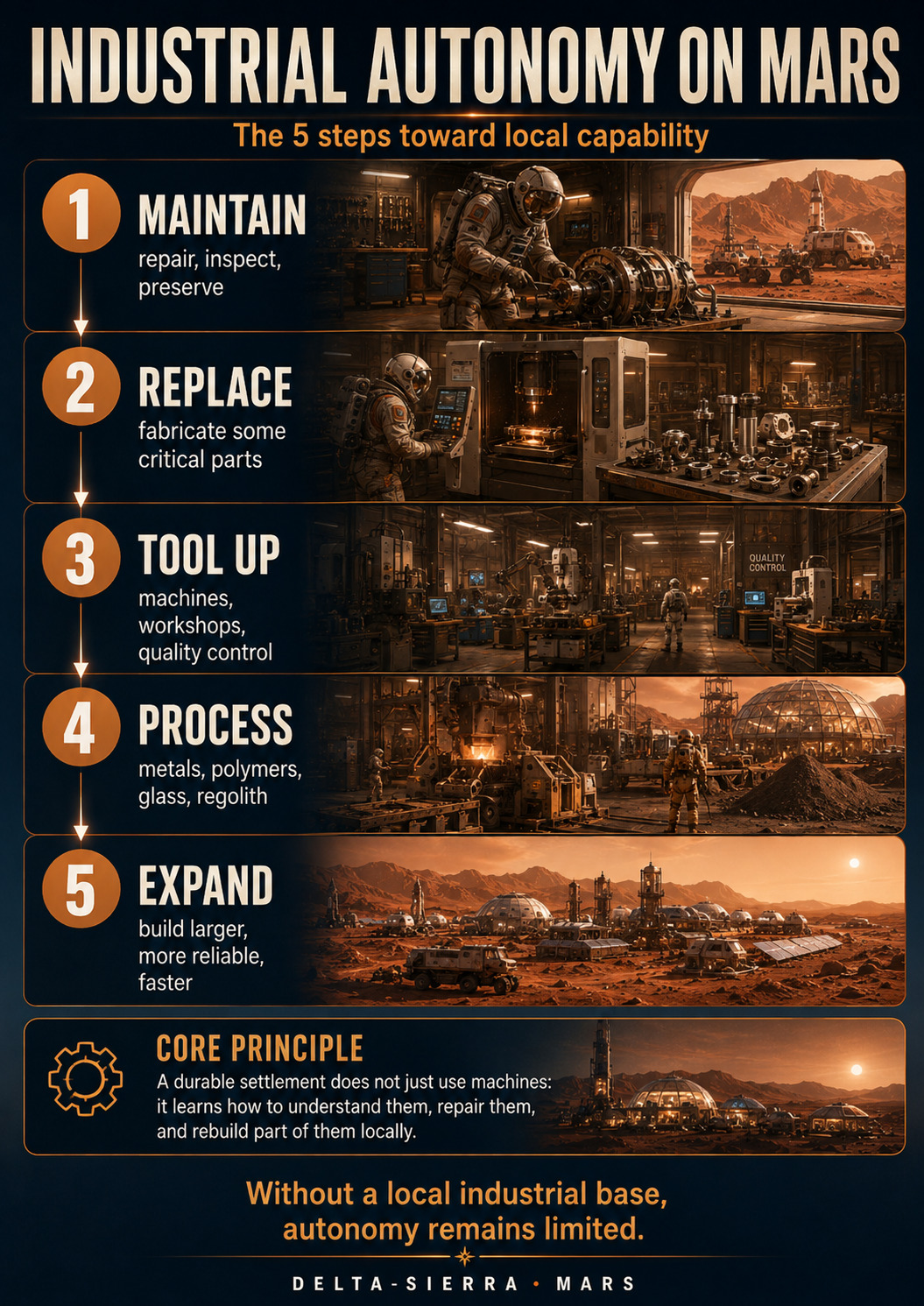
6. Mobility: distance costs more than propellant

A resource 30 km away implies routes, vehicles, energy, navigation, spares, rescue, and two-way movement. Catalogue rover range is insufficient.

Ask how far the vehicle can travel, lose a function, and still return or wait safely. Logistics evaluates complete missions with failure margin.

Premium poster on the stages of Martian industrial autonomy and local production. — Industrial autonomy is built in stages: stock, repair, manufacture, qualify, then transfer the know-how.

Quantified balance

Mobility must be sized with degraded return. Nominal rover range is not safe range after loss of a battery, wheel, sensor, or communication link. Architecture can use paired vehicles, caches, rescue robots, or distance limits depending on scenario.

Safe mobility radius

r_safe <= (v_degraded × t_degraded)/2 − distance_margin

1 — Concrete question: What operational question does this relation answer for safe mobility radius?
2 — Intuition without symbols: An excursion must remain returnable in degraded mode, so total range is split between outbound and return travel before subtracting margin.
3 — Quantities first: v_degraded is degraded speed, t_degraded available degraded duration, and distance_margin protected margin.
4 — Formula: r_safe <= (v_degraded × t_degraded)/2 − distance_margin
5 — Read aloud: Read the relation aloud term by term: r_safe <= (v_degraded × t_degraded)/2 − distance_margin.
6 — Symbols and meaning: v_degraded is degraded speed, t_degraded available degraded duration, and distance_margin protected margin.
7 — Pronunciation: The “Read aloud” line above is the oral reference for “Safe mobility radius”. Any subscript, exponent or grouping that changes the meaning of the relation should be spoken explicitly.
8 — Units: Speed times time gives distance; all distance terms must use the same unit.
9 — Convention: For “Safe mobility radius”, substitute values without changing the reference frame, time basis, system boundary or sign convention halfway through the calculation. Stated units: Speed times time gives distance; all distance terms must use the same unit.
10 — Why this operation: An excursion must remain returnable in degraded mode, so total range is split between outbound and return travel before subtracting margin.
11 — Assumptions: The relation “r_safe <= (v_degraded × t_degraded)/2 − distance_margin” applies here only to the scenario described by the card. Inputs must be mutually consistent and satisfy the physical assumptions associated with “Safe mobility radius”.
12 — Unit check: Speed times time gives distance; all distance terms must use the same unit. Verify that units reduce to the unit of the requested quantity.
13 — Numerical case: Teaching example: v_degraded = 5 km/h, t_degraded = 6 h, and distance_margin = 5 km gives r_safe ≤ (5×6)/2 − 5 = 10 km.
14 — Why the calculation works: An excursion must remain returnable in degraded mode, so total range is split between outbound and return travel before subtracting margin.
15 — Algebra check: Quick check: multiplying the result by the denominator should reconstruct the numerator of “Safe mobility radius” within rounding.
16 — Mental estimate: Before calculating “Safe mobility radius” precisely, round the inputs to one useful digit and predict the sign and order of magnitude. The detailed result should remain consistent with that estimate.
17 — Interpretation: The result is useful only as an operational statement about safe mobility radius under the declared assumptions.
18 — What the result does not prove: For “Safe mobility radius”, the number obtained answers only the model “r_safe <= (v_degraded × t_degraded)/2 − distance_margin” under the stated scenario. It does not by itself validate the input data or the model outside those conditions.
19 — Sensitivity: Vary one input at a time around the nominal case to identify what drives the result of “Safe mobility radius” and whether that variation can change the mission decision.
20 — Guided and autonomous practice: Guided exercise. Increase degraded speed by 10%, from 5 to 5.5 km/h, keeping 6 h and 5 km margin. Recompute safe radius.
Detailed guided correction — open after attempting
Detailed correction. r_safe ≤ (5.5×6)/2 − 5 = 33/2 − 5 = 16.5 − 5 = 11.5 km. The 0.5 km/h gain increases safe radius by 1.5 km while preserving the same distance margin.
Autonomous exercise. Build a second numerical scenario for “Safe mobility radius” by changing at least two inputs in r_safe <= (v_degraded × t_degraded)/2 − distance_margin. Compute the result, check units and order of magnitude, then state whether the mission decision should change.
Autonomous correction — specific criteria
Autonomous correction. The answer must show substitution into r_safe <= (v_degraded × t_degraded)/2 − distance_margin, produce a value with its unit or an explicit logical result, compare it with the reference case, and justify the following decision: Define the operational radius from degraded capability, not nominal vehicle range.
21 — Mission decision: Define the operational radius from degraded capability, not nominal vehicle range.

The one-half factor is only a round-trip intuition; terrain, detour, and rescue needs can require much larger margin.

Mobility case — rescue

A rover has 200 km nominal energy range but only 120 km with degraded battery and high heating load. A target 50 km away needs 100 km round trip before detour. With 20% detour the trip reaches 120 km and all margin disappears. Excursion limits must use degraded range, not nominal headline range.

Decision check. Mobility planning needs a rescue architecture. One option is paired crewed vehicles; another is an uncrewed recovery rover, route caches, or strict turn-back points. Each choice moves mass and complexity between the vehicle fleet and stationary infrastructure, so “range” is an architecture property rather than one battery number.

7. ISRU: demonstrate process, then design plant

MOXIE demonstrated oxygen production from Martian CO₂, with NASA reporting up to 12 g/h and 122 g total. A hypothetical 1 t/day demand is 41.7 kg/h, more than 3,400 times the demonstrated peak rate.

That ratio is not a plan for 3,400 copies. Industrial design changes compressors, cells, thermal rejection, power, storage, controls, maintenance, and availability. The correct status is small-scale principle demonstrated on Mars; industrialization remains to be engineered and qualified.

ISRU study — from demonstrated flow to guaranteed service

MOXIE demonstrated up to 12 g/h oxygen production on Mars and 122 g in total. Imagine a future nominal unit rated at 20 kg/h, a purely teaching value. At 90% availability across an 8,760-hour Earth year, output is 20×8,760×0.90 = 157,680 kg or 157.7 t/year. At 70%, it falls to 122.6 t/year. Twenty availability points are therefore worth about 35.0 t/year in this scenario.

This sensitivity is why industrial sizing includes maintenance, spares, contamination, cell life, compressors, storage, and power. Nameplate flow is not enough. Robust architecture separates instantaneous flow, availability, storage capacity, and cumulative demand. MOXIE supplies Mars proof of principle; availability of a future industrial plant remains a design variable.

Annual ISRU production

M_year = rate × 8,760 h × availability

1 — Concrete question: What operational question does this relation answer for annual isru production?
2 — Intuition without symbols: Real annual production starts from nominal throughput and credits only the fraction of the year that is actually productive.
3 — Quantities first: rate is nominal production per hour, availability productive fraction, and M_year annual output.
4 — Formula: M_year = rate × 8,760 h × availability
5 — Read aloud: Read the relation aloud term by term: M_year = rate × 8,760 h × availability.
6 — Symbols and meaning: rate is nominal production per hour, availability productive fraction, and M_year annual output.
7 — Pronunciation: The “Read aloud” line above is the oral reference for “Annual ISRU production”. Any subscript, exponent or grouping that changes the meaning of the relation should be spoken explicitly.
8 — Units: kg/h × h/year gives kg/year; availability is dimensionless.
9 — Convention: For “Annual ISRU production”, substitute values without changing the reference frame, time basis, system boundary or sign convention halfway through the calculation. Stated units: kg/h × h/year gives kg/year; availability is dimensionless.
10 — Why this operation: Real annual production starts from nominal throughput and credits only the fraction of the year that is actually productive.
11 — Assumptions: The relation “M_year = rate × 8,760 h × availability” applies here only to the scenario described by the card. Inputs must be mutually consistent and satisfy the physical assumptions associated with “Annual ISRU production”.
12 — Unit check: kg/h × h/year gives kg/year; availability is dimensionless. Verify that units reduce to the unit of the requested quantity.
13 — Numerical case: Teaching example: rate = 20 kg/h and availability = 0.90 gives M_year = 20 × 8,760 × 0.90 = 157,680 kg/year.
14 — Why the calculation works: Real annual production starts from nominal throughput and credits only the fraction of the year that is actually productive.
15 — Algebra check: Quick check: for any non-zero factor, dividing the result by that factor should recover the other expected contribution in “Annual ISRU production”.
16 — Mental estimate: Before calculating “Annual ISRU production” precisely, round the inputs to one useful digit and predict the sign and order of magnitude. The detailed result should remain consistent with that estimate.
17 — Interpretation: The result is useful only as an operational statement about annual isru production under the declared assumptions.
18 — What the result does not prove: For “Annual ISRU production”, the number obtained answers only the model “M_year = rate × 8,760 h × availability” under the stated scenario. It does not by itself validate the input data or the model outside those conditions.
19 — Sensitivity: Vary one input at a time around the nominal case to identify what drives the result of “Annual ISRU production” and whether that variation can change the mission decision.
20 — Guided and autonomous practice: Guided exercise. Increase rate by 10%, from 20 to 22 kg/h, keeping availability at 0.90. Recompute annual production.
Detailed guided correction — open after attempting
Detailed correction. M_year = 22 × 8,760 × 0.90 = 173,448 kg/year. The gain is 173,448 − 157,680 = 15,768 kg/year, exactly +10% because only rate changed.
Autonomous exercise. Build a second numerical scenario for “Annual ISRU production” by changing at least two inputs in M_year = rate × 8,760 h × availability. Compute the result, check units and order of magnitude, then state whether the mission decision should change.
Autonomous correction — specific criteria
Autonomous correction. The answer must show substitution into M_year = rate × 8,760 h × availability, produce a value with its unit or an explicit logical result, compare it with the reference case, and justify the following decision: Size reserves and redundancy from credible degraded annual production, not nameplate output.
21 — Mission decision: Size reserves and redundancy from credible degraded annual production, not nameplate output.

Degraded mode

ISRU means replacing an import with a complete local chain. Extraction alone is insufficient: capture, purification, conversion, storage, measurement, and maintenance are required. MOXIE demonstrated one oxygen-production step from Martian CO₂; MARS-C is a 2026 active technology project, not an operational plant.

Generic annual production

annual_production = rate × availability × 8,760 h

1 — Concrete question: What operational question does this relation answer for generic annual production?
2 — Intuition without symbols: The same availability budget applies to any machine whose nominal rate is not available continuously.
3 — Quantities first: rate is nominal throughput and availability the fraction of the year that can actually produce.
4 — Formula: annual_production = rate × availability × 8,760 h
5 — Read aloud: Read the relation aloud term by term: annual_production = rate × availability × 8,760 h.
6 — Symbols and meaning: rate is nominal throughput and availability the fraction of the year that can actually produce.
7 — Pronunciation: The “Read aloud” line above is the oral reference for “Generic annual production”. Any subscript, exponent or grouping that changes the meaning of the relation should be spoken explicitly.
8 — Units: A per-hour rate multiplied by annual hours gives per-year output.
9 — Convention: For “Generic annual production”, substitute values without changing the reference frame, time basis, system boundary or sign convention halfway through the calculation. Stated units: A per-hour rate multiplied by annual hours gives per-year output.
10 — Why this operation: The same availability budget applies to any machine whose nominal rate is not available continuously.
11 — Assumptions: The relation “annual_production = rate × availability × 8,760 h” applies here only to the scenario described by the card. Inputs must be mutually consistent and satisfy the physical assumptions associated with “Generic annual production”.
12 — Unit check: A per-hour rate multiplied by annual hours gives per-year output. Verify that units reduce to the unit of the requested quantity.
13 — Numerical case: Teaching example: rate = 5 kg/h and availability = 0.80 gives annual_production = 5 × 0.80 × 8,760 = 35,040 kg/year.
14 — Why the calculation works: The same availability budget applies to any machine whose nominal rate is not available continuously.
15 — Algebra check: Quick check: for any non-zero factor, dividing the result by that factor should recover the other expected contribution in “Generic annual production”.
16 — Mental estimate: Before calculating “Generic annual production” precisely, round the inputs to one useful digit and predict the sign and order of magnitude. The detailed result should remain consistent with that estimate.
17 — Interpretation: The result is useful only as an operational statement about generic annual production under the declared assumptions.
18 — What the result does not prove: For “Generic annual production”, the number obtained answers only the model “annual_production = rate × availability × 8,760 h” under the stated scenario. It does not by itself validate the input data or the model outside those conditions.
19 — Sensitivity: Vary one input at a time around the nominal case to identify what drives the result of “Generic annual production” and whether that variation can change the mission decision.
20 — Guided and autonomous practice: Guided exercise. Increase availability by 10% relatively, from 0.80 to 0.88, at the same rate. Recompute production.
Detailed guided correction — open after attempting
Detailed correction. annual_production = 5 × 0.88 × 8,760 = 38,544 kg/year. The gain is 3,504 kg/year, or +10% relative to the initial 35,040 kg/year.
Autonomous exercise. Build a second numerical scenario for “Generic annual production” by changing at least two inputs in annual_production = rate × availability × 8,760 h. Compute the result, check units and order of magnitude, then state whether the mission decision should change.
Autonomous correction — specific criteria
Autonomous correction. The answer must show substitution into annual_production = rate × availability × 8,760 h, produce a value with its unit or an explicit logical result, compare it with the reference case, and justify the following decision: Compare annual demand with annual production plus explicit margin before relying on local supply.
21 — Mission decision: Compare annual demand with annual production plus explicit margin before relying on local supply.

Scaling must be demonstrated in power, lifetime, maintenance, and purity, not merely nominal flow rate.

ISRU case — availability

A nominal 2 kg O₂/h plant operating 70% of the year produces 2×8,760×0.70=12,264 kg/year. At 90% it produces 15,768 kg/year, a 3.504 t difference. Maintainability can therefore be worth several tonnes per year without changing nominal flow by one gram.

8. Workshop, metrology, spare parts

A manufactured part is not automatically qualified for critical service. Material, dimensions, tolerances, surface state, treatments, and defects must be measured. NIST’s 2026 in-situ metrology work explicitly connects measurement with qualification and certification for metal additive manufacturing.

A Mars workshop therefore needs machines, instruments, standards, material data, and acceptance criteria. A simple bracket may become local while a bearing, sensor, or electronic component stays imported.

Workshop study — machine capacity and qualification

Suppose a workshop has one critical machine available 20 h/day after maintenance, tool changes, and checks. Three part families require 6 h, 8 h, and 10 h of machine time per batch. One day cannot produce all three batches because demand totals 24 h. The bottleneck is not “owning a printer” but scheduling a scarce qualified resource.

If a life-critical repair needing 7 h arrives, it must displace another job or wait. A second machine doubles capacity only if operators, feedstock, metrology, power, and tooling also scale. NIST’s 2026 workshop on in-situ metrology for metal additive manufacturing explicitly links measurement with qualification and certification. A part leaving a machine is not automatically an acceptable life-critical part.

Daily workshop workload

demand = 6 + 8 + 10

1 — Concrete question: What operational question does this relation answer for daily workshop workload?
2 — Intuition without symbols: Jobs competing for the same machine resource are added before comparing them with available daily capacity.
3 — Quantities first: Each term is machine-hours/day required by one work family; demand is total machine-hours/day.
4 — Formula: demand = 6 + 8 + 10
5 — Read aloud: Read the relation aloud term by term: demand = 6 + 8 + 10.
6 — Symbols and meaning: Each term is machine-hours/day required by one work family; demand is total machine-hours/day.
7 — Pronunciation: The “Read aloud” line above is the oral reference for “Daily workshop workload”. Any subscript, exponent or grouping that changes the meaning of the relation should be spoken explicitly.
8 — Units: All workload terms use machine-hours per day.
9 — Convention: For “Daily workshop workload”, substitute values without changing the reference frame, time basis, system boundary or sign convention halfway through the calculation. Stated units: All workload terms use machine-hours per day.
10 — Why this operation: Jobs competing for the same machine resource are added before comparing them with available daily capacity.
11 — Assumptions: The relation “demand = 6 + 8 + 10” applies here only to the scenario described by the card. Inputs must be mutually consistent and satisfy the physical assumptions associated with “Daily workshop workload”.
12 — Unit check: All workload terms use machine-hours per day. Verify that units reduce to the unit of the requested quantity.
13 — Numerical case: Teaching example: three job families require 6 h, 8 h, and 10 machine-h/day, so demand = 24 h/day. Against 20 h/day usable capacity, deficit is 4 h/day.
14 — Why the calculation works: Jobs competing for the same machine resource are added before comparing them with available daily capacity.
15 — Algebra check: Quick check: subtracting one contribution from the total should recover the sum of the remaining contributions in “Daily workshop workload”.
16 — Mental estimate: Before calculating “Daily workshop workload” precisely, round the inputs to one useful digit and predict the sign and order of magnitude. The detailed result should remain consistent with that estimate.
17 — Interpretation: The result is useful only as an operational statement about daily workshop workload under the declared assumptions.
18 — What the result does not prove: For “Daily workshop workload”, the number obtained answers only the model “demand = 6 + 8 + 10” under the stated scenario. It does not by itself validate the input data or the model outside those conditions.
19 — Sensitivity: Vary one input at a time around the nominal case to identify what drives the result of “Daily workshop workload” and whether that variation can change the mission decision.
20 — Guided and autonomous practice: Guided exercise. Increase the second demand by 10%, from 8 to 8.8 h/day, with other needs and 20 h/day capacity unchanged. Recompute workload and deficit.
Detailed guided correction — open after attempting
Detailed correction. demand = 6 + 8.8 + 10 = 24.8 h/day. Deficit = 24.8 − 20 = 4.8 h/day. The 0.8 h increase in one family passes directly into daily backlog: 4.0 → 4.8 h/day.
Autonomous exercise. Build a second numerical scenario for “Daily workshop workload” by changing at least two inputs in demand = 6 + 8 + 10. Compute the result, check units and order of magnitude, then state whether the mission decision should change.
Autonomous correction — specific criteria
Autonomous correction. The answer must show substitution into demand = 6 + 8 + 10, produce a value with its unit or an explicit logical result, compare it with the reference case, and justify the following decision: Prioritize work or add capacity when sustained demand exceeds available machine time.
21 — Mission decision: Prioritize work or add capacity when sustained demand exceeds available machine time.

Safety reading

A workshop is not an isolated printer: it needs feedstock, preparation, machine tools, metrology, qualification, design data, operators, and configuration control. NIST’s 2026 in-situ metrology workshop highlights measurement, qualification, and certification as central metal-additive challenges.

Qualified deliverable capacity

qualified_capacity = rate × availability × yield × acceptance_rate

1 — Concrete question: What operational question does this relation answer for qualified deliverable capacity?
2 — Intuition without symbols: Useful capacity is nominal rate reduced by availability, process yield, and product acceptance losses.
3 — Quantities first: rate is nominal throughput; availability, yield and acceptance_rate are dimensionless fractions.
4 — Formula: qualified_capacity = rate × availability × yield × acceptance_rate
5 — Read aloud: Read the relation aloud term by term: qualified_capacity = rate × availability × yield × acceptance_rate.
6 — Symbols and meaning: rate is nominal throughput; availability, yield and acceptance_rate are dimensionless fractions.
7 — Pronunciation: The “Read aloud” line above is the oral reference for “Qualified deliverable capacity”. Any subscript, exponent or grouping that changes the meaning of the relation should be spoken explicitly.
8 — Units: The result keeps the throughput unit of the nominal rate.
9 — Convention: For “Qualified deliverable capacity”, substitute values without changing the reference frame, time basis, system boundary or sign convention halfway through the calculation. Stated units: The result keeps the throughput unit of the nominal rate.
10 — Why this operation: Useful capacity is nominal rate reduced by availability, process yield, and product acceptance losses.
11 — Assumptions: The relation “qualified_capacity = rate × availability × yield × acceptance_rate” applies here only to the scenario described by the card. Inputs must be mutually consistent and satisfy the physical assumptions associated with “Qualified deliverable capacity”.
12 — Unit check: The result keeps the throughput unit of the nominal rate. Verify that units reduce to the unit of the requested quantity.
13 — Numerical case: Teaching example: rate = 100 kg/h, availability = 0.90, yield = 0.80, and acceptance_rate = 0.95 gives qualified_capacity = 68.4 kg/h.
14 — Why the calculation works: Useful capacity is nominal rate reduced by availability, process yield, and product acceptance losses.
15 — Algebra check: Quick check: for any non-zero factor, dividing the result by that factor should recover the other expected contribution in “Qualified deliverable capacity”.
16 — Mental estimate: Before calculating “Qualified deliverable capacity” precisely, round the inputs to one useful digit and predict the sign and order of magnitude. The detailed result should remain consistent with that estimate.
17 — Interpretation: The result is useful only as an operational statement about qualified deliverable capacity under the declared assumptions.
18 — What the result does not prove: For “Qualified deliverable capacity”, the number obtained answers only the model “qualified_capacity = rate × availability × yield × acceptance_rate” under the stated scenario. It does not by itself validate the input data or the model outside those conditions.
19 — Sensitivity: Vary one input at a time around the nominal case to identify what drives the result of “Qualified deliverable capacity” and whether that variation can change the mission decision.
20 — Guided and autonomous practice: Guided exercise. Increase nominal rate by 10%, from 100 to 110 kg/h, leaving the three fractions unchanged. Recompute qualified capacity.
Detailed guided correction — open after attempting
Detailed correction. qualified_capacity = 110 × 0.90 × 0.80 × 0.95 = 75.24 kg/h. The gain is 6.84 kg/h, or +10%, because availability, yield, and acceptance factors remain constant.
Autonomous exercise. Build a second numerical scenario for “Qualified deliverable capacity” by changing at least two inputs in qualified_capacity = rate × availability × yield × acceptance_rate. Compute the result, check units and order of magnitude, then state whether the mission decision should change.
Autonomous correction — specific criteria
Autonomous correction. The answer must show substitution into qualified_capacity = rate × availability × yield × acceptance_rate, produce a value with its unit or an explicit logical result, compare it with the reference case, and justify the following decision: Commit production using qualified capacity rather than nominal rate.
21 — Mission decision: Commit production using qualified capacity rather than nominal rate.

A produced part is not yet released for service until critical characteristics are verified.

Workshop case — qualification

A printer makes 10 parts/h but 15% fail inspection and 10% of time is lost to changeover. Over 16 scheduled hours, accepted output≈10×16×0.90×0.85=122 parts. The raw “160 parts” figure overstates useful capacity by ignoring support time and acceptance.

9. Population and skill depth

Four people are a mission team; twenty allow more specialties; one hundred begin to support permanent services; one thousand can sustain training pipelines but require much more complex infrastructure.

Headcount alone is insufficient. Track critical skills, available labor, training of replacements, and maintenance burden. A durable society must reproduce knowledge as well as parts.

System intuition

Population growth requires skill depth, not simply more people. A critical function needs backups, hands-on training, documentation, and a training time compatible with crew turnover.

Critical-skill coverage

skill_coverage = qualified_people × individual_availability

1 — Concrete question: What operational question does this relation answer for critical-skill coverage?
2 — Intuition without symbols: Counting trained people is not enough: real coverage also depends on their simultaneous availability.
3 — Quantities first: qualified_people is the number of competent people and individual_availability the usable fraction of their time.
4 — Formula: skill_coverage = qualified_people × individual_availability
5 — Read aloud: Read the relation aloud term by term: skill_coverage = qualified_people × individual_availability.
6 — Symbols and meaning: qualified_people is the number of competent people and individual_availability the usable fraction of their time.
7 — Pronunciation: The “Read aloud” line above is the oral reference for “Critical-skill coverage”. Any subscript, exponent or grouping that changes the meaning of the relation should be spoken explicitly.
8 — Units: The result is an equivalent available qualified-person capacity.
9 — Convention: For “Critical-skill coverage”, substitute values without changing the reference frame, time basis, system boundary or sign convention halfway through the calculation. Stated units: The result is an equivalent available qualified-person capacity.
10 — Why this operation: Counting trained people is not enough: real coverage also depends on their simultaneous availability.
11 — Assumptions: The relation “skill_coverage = qualified_people × individual_availability” applies here only to the scenario described by the card. Inputs must be mutually consistent and satisfy the physical assumptions associated with “Critical-skill coverage”.
12 — Unit check: The result is an equivalent available qualified-person capacity. Verify that units reduce to the unit of the requested quantity.
13 — Numerical case: Teaching example: 3 qualified people at individual availability 0.80 gives skill_coverage = 3 × 0.80 = 2.4 equivalent available qualified people.
14 — Why the calculation works: Counting trained people is not enough: real coverage also depends on their simultaneous availability.
15 — Algebra check: Quick check: for any non-zero factor, dividing the result by that factor should recover the other expected contribution in “Critical-skill coverage”.
16 — Mental estimate: Before calculating “Critical-skill coverage” precisely, round the inputs to one useful digit and predict the sign and order of magnitude. The detailed result should remain consistent with that estimate.
17 — Interpretation: The result is useful only as an operational statement about critical-skill coverage under the declared assumptions.
18 — What the result does not prove: For “Critical-skill coverage”, the number obtained answers only the model “skill_coverage = qualified_people × individual_availability” under the stated scenario. It does not by itself validate the input data or the model outside those conditions.
19 — Sensitivity: Vary one input at a time around the nominal case to identify what drives the result of “Critical-skill coverage” and whether that variation can change the mission decision.
20 — Guided and autonomous practice: Guided exercise. Increase individual availability by 10% relatively, from 0.80 to 0.88, with 3 qualified people unchanged. Recompute coverage.
Detailed guided correction — open after attempting
Detailed correction. skill_coverage = 3 × 0.88 = 2.64 equivalent people. The gain is 0.24 equivalent, or +10% relative to the initial 2.4. This does not create a fourth physical person.
Autonomous exercise. Build a second numerical scenario for “Critical-skill coverage” by changing at least two inputs in skill_coverage = qualified_people × individual_availability. Compute the result, check units and order of magnitude, then state whether the mission decision should change.
Autonomous correction — specific criteria
Autonomous correction. The answer must show substitution into skill_coverage = qualified_people × individual_availability, produce a value with its unit or an explicit logical result, compare it with the reference case, and justify the following decision: Require independent qualified backup for every function whose absence could stop the mission.
21 — Mission decision: Require independent qualified backup for every function whose absence could stop the mission.

A theoretical skill unused for a long time may not equal active operator capability; recurrent drills are part of human maintenance.

Skills case — crew rotation

A critical function has three specialists. One is on a long EVA, one is ill, and the third must supervise another emergency. Nominal “three qualified people” becomes zero practical availability. Planning must combine skill matrix, scheduling, simultaneous unavailability, and cross-training.

Decision check. Skill depth can be visualized as a matrix of people versus functions, with levels such as awareness, supervised operation, independent operation, diagnosis, and instructor. The goal is not to make everyone expert in everything; it is to prevent one absence from erasing the only local capability to restore a vital system.

10. Operational governance and safety

Life-critical systems need clear authority: who can shut down a plant, reject a water batch, draw emergency reserve, or isolate a zone? These are safety mechanisms before they are a full political constitution.

Broader institutional choices come later: resource allocation, investment, ownership, emergency duties, transparency, conflict. Separate constraints imposed by physics from choices created by institutions.

Quantified balance

Operational governance turns principles into concrete authorities: stop a line, isolate a habitat, use a reserve, change configuration, accept a part, or postpone an EVA. Rules need traceability while retaining a fast emergency path.

Safe and traceable decision

safe decision <=> authority AND information AND threshold AND trace

1 — Concrete question: What operational question does this relation answer for safe and traceable decision?
2 — Intuition without symbols: A critical decision is safe only when the right authority has the required information, an explicit threshold, and a verifiable record.
3 — Quantities first: The four terms are mandatory logical conditions rather than additive numerical quantities.
4 — Formula: safe decision <=> authority AND information AND threshold AND trace
5 — Read aloud: Read the relation aloud term by term: safe decision <=> authority AND information AND threshold AND trace.
6 — Symbols and meaning: The four terms are mandatory logical conditions rather than additive numerical quantities.
7 — Pronunciation: The “Read aloud” line above is the oral reference for “Safe and traceable decision”. Any subscript, exponent or grouping that changes the meaning of the relation should be spoken explicitly.
8 — Units: This is a logical rule with no single physical unit.
9 — Convention: For “Safe and traceable decision”, substitute values without changing the reference frame, time basis, system boundary or sign convention halfway through the calculation. Stated units: This is a logical rule with no single physical unit.
10 — Why this operation: A critical decision is safe only when the right authority has the required information, an explicit threshold, and a verifiable record.
11 — Assumptions: The relation “safe decision <=> authority AND information AND threshold AND trace” applies here only to the scenario described by the card. Inputs must be mutually consistent and satisfy the physical assumptions associated with “Safe and traceable decision”.
12 — Unit check: This is a logical rule with no single physical unit. Verify that units reduce to the unit of the requested quantity.
13 — Numerical case: Teaching example: of 4 mandatory conditions, authority = yes, information = yes, threshold = no, trace = yes. Even though 3 of 4 are present, safe decision remains FALSE because the rule uses AND across all four conditions.
14 — Why the calculation works: A critical decision is safe only when the right authority has the required information, an explicit threshold, and a verifiable record.
15 — Algebra check: Quick check: invert “safe decision <=> authority AND information AND threshold AND trace” when possible, or use a second calculation path, and confirm the same order of magnitude for “Safe and traceable decision”.
16 — Mental estimate: Before calculating “Safe and traceable decision” precisely, round the inputs to one useful digit and predict the sign and order of magnitude. The detailed result should remain consistent with that estimate.
17 — Interpretation: The result is useful only as an operational statement about safe and traceable decision under the declared assumptions.
18 — What the result does not prove: For “Safe and traceable decision”, the number obtained answers only the model “safe decision <=> authority AND information AND threshold AND trace” under the stated scenario. It does not by itself validate the input data or the model outside those conditions.
19 — Sensitivity: Vary one input at a time around the nominal case to identify what drives the result of “Safe and traceable decision” and whether that variation can change the mission decision.
20 — Guided and autonomous practice: Guided exercise. The missing threshold is then formalized and validated, making all four conditions yes. Does the decision now satisfy the rule?
Detailed guided correction — open after attempting
Detailed correction. With authority = yes, information = yes, threshold = yes, and trace = yes, all 4 mandatory conditions are true, so the AND expression becomes true. The 4/4 count illustrates completeness; it does not turn the rule into a compensatory score.
Autonomous exercise. Build a second numerical scenario for “Safe and traceable decision” by changing at least two inputs in safe decision <=> authority AND information AND threshold AND trace. Compute the result, check units and order of magnitude, then state whether the mission decision should change.
Autonomous correction — specific criteria
Autonomous correction. The answer must show substitution into safe decision <=> authority AND information AND threshold AND trace, produce a value with its unit or an explicit logical result, compare it with the reference case, and justify the following decision: Reject critical decisions based on implicit authority or an unwritten threshold.
21 — Mission decision: Reject critical decisions based on implicit authority or an unwritten threshold.

A procedure requiring immediate Earth communication is not robust to Mars delay and outages.

Governance case — plant shutdown

An ISRU line exceeds a temperature threshold but shutdown would sacrifice needed oxygen production. Rules must specify who decides, which threshold forces automatic shutdown, what reserve survives the outage, and how any override is recorded. Without those elements, “safety first” remains an intention rather than an executable rule.

Decision check. Operational governance should also define evidence thresholds. A technician may be allowed to stop a machine from one alarming sensor but require two independent checks before permanently rejecting a batch. Different actions justify different standards of evidence because delay and false action have different consequences.

11. Physical economy: mass, energy, machine time

Before currency, a settlement has a physical economy. A part consumes material, kWh, machine hours, human time, and risk. Saving one imported kilogram may be less valuable than tying up the rarest machine for twenty hours.

Indicators such as imported kg, kWh, availability, days of inventory, maintenance hours, and repair time compare architectures without pretending to forecast an entire future economy.

Degraded mode

Physical economy reveals bottlenecks before money is discussed: available energy, imported mass, machine hours, crew time, pressurized area, and inventory. A currency or price can allocate scarcity but cannot create additional kilowatt-hours.

Bottleneck-limited capacity

capacity = min(resource, energy, machine, operator, metrology)

1 — Concrete question: What operational question does this relation answer for bottleneck-limited capacity?
2 — Intuition without symbols: A chain cannot deliver more than its most limiting link once every capacity is converted to the same basis.
3 — Quantities first: Each branch is an equivalent capacity for the same product or service; min selects the limiting value.
4 — Formula: capacity = min(resource, energy, machine, operator, metrology)
5 — Read aloud: Read the relation aloud term by term: capacity = min(resource, energy, machine, operator, metrology).
6 — Symbols and meaning: Each branch is an equivalent capacity for the same product or service; min selects the limiting value.
7 — Pronunciation: The “Read aloud” line above is the oral reference for “Bottleneck-limited capacity”. Any subscript, exponent or grouping that changes the meaning of the relation should be spoken explicitly.
8 — Units: All compared capacities must use one common throughput unit.
9 — Convention: For “Bottleneck-limited capacity”, substitute values without changing the reference frame, time basis, system boundary or sign convention halfway through the calculation. Stated units: All compared capacities must use one common throughput unit.
10 — Why this operation: A chain cannot deliver more than its most limiting link once every capacity is converted to the same basis.
11 — Assumptions: The relation “capacity = min(resource, energy, machine, operator, metrology)” applies here only to the scenario described by the card. Inputs must be mutually consistent and satisfy the physical assumptions associated with “Bottleneck-limited capacity”.
12 — Unit check: All compared capacities must use one common throughput unit. Verify that units reduce to the unit of the requested quantity.
13 — Numerical case: Teaching example: equivalent capacities of 80, 70, 90, 85, and 75 units/h gives capacity = min(...) = 70 units/h; energy is the bottleneck.
14 — Why the calculation works: A chain cannot deliver more than its most limiting link once every capacity is converted to the same basis.
15 — Algebra check: Quick check: converting the logarithmic result back to the corresponding ratio should recover the scale of the input used in “Bottleneck-limited capacity”.
16 — Mental estimate: Before calculating “Bottleneck-limited capacity” precisely, round the inputs to one useful digit and predict the sign and order of magnitude. The detailed result should remain consistent with that estimate.
17 — Interpretation: The result is useful only as an operational statement about bottleneck-limited capacity under the declared assumptions.
18 — What the result does not prove: For “Bottleneck-limited capacity”, the number obtained answers only the model “capacity = min(resource, energy, machine, operator, metrology)” under the stated scenario. It does not by itself validate the input data or the model outside those conditions.
19 — Sensitivity: Vary one input at a time around the nominal case to identify what drives the result of “Bottleneck-limited capacity” and whether that variation can change the mission decision.
20 — Guided and autonomous practice: Guided exercise. Increase energy capacity by 10%, from 70 to 77 units/h, keeping other values unchanged. Recompute system capacity and identify the new bottleneck.
Detailed guided correction — open after attempting
Detailed correction. Capacities become 80, 77, 90, 85, and 75 units/h. The minimum is now 75 units/h, so metrology becomes the new bottleneck. A 10% energy improvement therefore raises system output by only 5 units/h, from 70 to 75.
Autonomous exercise. Build a second numerical scenario for “Bottleneck-limited capacity” by changing at least two inputs in capacity = min(resource, energy, machine, operator, metrology). Compute the result, check units and order of magnitude, then state whether the mission decision should change.
Autonomous correction — specific criteria
Autonomous correction. The answer must show substitution into capacity = min(resource, energy, machine, operator, metrology), produce a value with its unit or an explicit logical result, compare it with the reference case, and justify the following decision: Improve the real bottleneck before adding capacity to a branch that is already non-limiting.
21 — Mission decision: Improve the real bottleneck before adding capacity to a branch that is already non-limiting.

The chain minimum dominates: improving a non-bottleneck station may not increase output.

Physical-economy case — bottleneck

The workshop has feedstock for 500 parts and energy for 700, but metrology can inspect only 80 parts/day. Production at 150 parts/day does not raise qualified output above 80 while inspection is the bottleneck. The useful investment may therefore be a measurement station rather than a second production machine.

Decision check. A bottleneck analysis should be repeated after every major expansion. Adding population changes demand, but adding one new machine can shift the limiting factor to power, operator time, metrology, storage, or feedstock. The useful question is always “what constrains qualified output now?” rather than “which subsystem looks busiest?”

12. Failure scenarios as design tools

A useful scenario is not “everything fails.” Combine plausible events: one cargo lost, water pump unavailable, post-EVA dust, a metrology instrument offline, and communication delay. The goal is to expose dependencies.

A good scenario produces action: increase a reserve, isolate an interface, simplify repair, train a second specialist, or add independent sensing. Failure analysis becomes design work.

Safety reading

Failure scenarios should expose couplings: power plus water, mobility plus radiation, workshop plus spare stock, sensor plus common software. Examine detection, isolation, degraded mode, repair time, and return to a qualified state.

Degraded-mode survival margin

survival_margin = degraded_endurance − recovery_time

1 — Concrete question: What operational question does this relation answer for degraded-mode survival margin?
2 — Intuition without symbols: Raw endurance is not margin: first reserve the full time needed to recover or reach a safe state.
3 — Quantities first: degraded_endurance is sustainable degraded time, recovery_time the time needed for recovery, and survival_margin the remaining protected time.
4 — Formula: survival_margin = degraded_endurance − recovery_time
5 — Read aloud: Read the relation aloud term by term: survival_margin = degraded_endurance − recovery_time.
6 — Symbols and meaning: degraded_endurance is sustainable degraded time, recovery_time the time needed for recovery, and survival_margin the remaining protected time.
7 — Pronunciation: The “Read aloud” line above is the oral reference for “Degraded-mode survival margin”. Any subscript, exponent or grouping that changes the meaning of the relation should be spoken explicitly.
8 — Units: All three quantities are times in the same unit.
9 — Convention: For “Degraded-mode survival margin”, substitute values without changing the reference frame, time basis, system boundary or sign convention halfway through the calculation. Stated units: All three quantities are times in the same unit.
10 — Why this operation: Raw endurance is not margin: first reserve the full time needed to recover or reach a safe state.
11 — Assumptions: The relation “survival_margin = degraded_endurance − recovery_time” applies here only to the scenario described by the card. Inputs must be mutually consistent and satisfy the physical assumptions associated with “Degraded-mode survival margin”.
12 — Unit check: All three quantities are times in the same unit. Verify that units reduce to the unit of the requested quantity.
13 — Numerical case: Teaching example: degraded_endurance = 36 h and recovery_time = 12 h gives survival_margin = 24 h.
14 — Why the calculation works: Raw endurance is not margin: first reserve the full time needed to recover or reach a safe state.
15 — Algebra check: Quick check: adding the subtracted term back to the result should reconstruct the starting quantity in “Degraded-mode survival margin”.
16 — Mental estimate: Before calculating “Degraded-mode survival margin” precisely, round the inputs to one useful digit and predict the sign and order of magnitude. The detailed result should remain consistent with that estimate.
17 — Interpretation: The result is useful only as an operational statement about degraded-mode survival margin under the declared assumptions.
18 — What the result does not prove: For “Degraded-mode survival margin”, the number obtained answers only the model “survival_margin = degraded_endurance − recovery_time” under the stated scenario. It does not by itself validate the input data or the model outside those conditions.
19 — Sensitivity: Vary one input at a time around the nominal case to identify what drives the result of “Degraded-mode survival margin” and whether that variation can change the mission decision.
20 — Guided and autonomous practice: Guided exercise. Increase recovery time by 10%, from 12 to 13.2 h, with degraded endurance unchanged. Recompute margin.
Detailed guided correction — open after attempting
Detailed correction. survival_margin = 36 − 13.2 = 22.8 h. The 1.2 h increase in recovery time removes exactly 1.2 h from margin: 24 → 22.8 h. A positive margin is not automatically sufficient if fallback requires more than 22.8 h.
Autonomous exercise. Build a second numerical scenario for “Degraded-mode survival margin” by changing at least two inputs in survival_margin = degraded_endurance − recovery_time. Compute the result, check units and order of magnitude, then state whether the mission decision should change.
Autonomous correction — specific criteria
Autonomous correction. The answer must show substitution into survival_margin = degraded_endurance − recovery_time, produce a value with its unit or an explicit logical result, compare it with the reference case, and justify the following decision: Escalate when margin falls below the time required for a credible fallback option.
21 — Mission decision: Escalate when margin falls below the time required for a credible fallback option.

Positive margin in a nominal scenario is insufficient when repair-time uncertainty is of the same order as the margin.

Combined failure — power plus water

A generator failure sheds industrial loads while the water processor needs heater power to restart. If emergency mode did not reserve that restart power, water remains unavailable even after nominal generation returns. Combined scenarios must therefore follow the time sequence of functions, not merely a list of failed components.

Decision check. Failure scenarios become more realistic when they include recovery order. Restoring power does not instantly restore water if heaters, pumps, and quality checks must restart in sequence. The timeline should therefore include detection, isolation, minimum safe state, repair, restart, verification, and replenishment of depleted reserves.

13. Four scales, four architectures

Scale	Character	Question
4	integrated mission	Does one fault remain survivable?
20	specialized outpost	Which skills/spares need duplication?
100	permanent base	Which services become infrastructure?
1,000	industrial society	Which local chains replace imports?

Progression is not automatic. One hundred people can still depend on one imported component. Scale reveals architectural transitions; it does not provide a colonization date.

14. Final project: a 100-person base

Build a ten-function matrix: power, water, atmosphere, food, habitat, health, mobility, communications, workshop, spares. For each, record nominal capability, capability after one fault, emergency stock, repair time, and common dependencies.

The project succeeds when each function can be explained as ready, acceptable in degraded mode, or blocking, with missing evidence clearly identified. A credible architecture is a network of explicit functions and limits, not a collection of impressive technologies.

Final project — physical architecture of a 100-person base

Start with ten functions: energy, water, atmosphere, food, habitat, health, mobility, communications, workshop, and spares. For each, record nominal capacity and, more importantly, capacity after one fault. A 100-person base with 500 kW generation but only 120 kWh storage has a different resilience profile from one with the same generation and several days of reserve. Quantities are not interchangeable: power, energy, flow, inventory mass, and repair time answer different questions.

For water, use a teaching net loss of 40 kg/day after recovery. Thirty days of makeup is 1,200 kg. A ninety-day strategic reserve is 3.6 t. If loss doubles during degraded operation, a nominal ninety-day reserve becomes forty-five days. Inventory has not changed; endurance changed because flow changed. The base must therefore monitor loss trends as well as tank levels.

For construction, a 300 t regolith job at 250 kg/h is 1,200 productive hours. If two identical machines are genuinely independent, nominal throughput may approach 500 kg/h. Yet one maintenance workshop, one charging system, or one shared wear part can limit the gain. For every capacity, record the dependency that can make failures common. That column often reveals more than the machine count.

For industry, assume one critical machine tool is available 18 h/day and planned demand is 15 h/day. Nominal utilization is 83%. An unexpected eight-hour repair cannot be absorbed the same day without delay. Sufficient average capacity can still lack time margin. Add a backlog indicator measured in waiting machine-hours. If backlog rises for several days, the workshop is structurally under-capacity even though no machine is completely failed.

For skills, count more than people. List functions in which only one specialist can authorize or perform an operation: surgery, quality control, high voltage, critical software, chemistry, compressor maintenance. A hundred-person settlement can be demographically large and technically fragile. The plan needs apprenticeship, documentation, simulators, drills, and protected training time. Reproducing skills is infrastructure just as surely as inventorying spare parts.

Finish with three combined scenarios: loss of an annual cargo, a 72-hour ECLSS train outage, and simultaneous loss of a metrology machine. For each, identify functions maintained, degraded services, inventories consumed, recovery time, and the decision that becomes irreversible. The goal is not to predict the first Mars city but to show that settlement architecture can be discussed through balances, dependencies, degraded modes, and evidence.

Function	Useful measure	Resilience question
Energy	kW + kWh + availability	how long after generation loss?
Water	kg/day loss + reserve tonnes	what endurance at degraded flow?
Workshop	machine h/day + backlog	which repair delays others?
Skills	qualified people per function	which task has one human point of failure?

Integrated sustainability dashboard

endurance = stock/loss ; utilization = demand/capacity ; availability != nameplate capacity

1 — Concrete question: What operational question does this relation answer for integrated sustainability dashboard?
2 — Intuition without symbols: Sustainability combines at least reserve endurance, workload, and real equipment availability; no single indicator is sufficient.
3 — Quantities first: Stock and loss give endurance; demand and capacity give utilization; availability describes real access to nominal capacity.
4 — Formula: endurance = stock/loss ; utilization = demand/capacity ; availability != nameplate capacity
5 — Read aloud: Read the relation aloud term by term: endurance = stock/loss ; utilization = demand/capacity ; availability != nameplate capacity.
6 — Symbols and meaning: Stock and loss give endurance; demand and capacity give utilization; availability describes real access to nominal capacity.
7 — Pronunciation: The “Read aloud” line above is the oral reference for “Integrated sustainability dashboard”. Any subscript, exponent or grouping that changes the meaning of the relation should be spoken explicitly.
8 — Units: Endurance is time; utilization and availability are dimensionless ratios.
9 — Convention: For “Integrated sustainability dashboard”, substitute values without changing the reference frame, time basis, system boundary or sign convention halfway through the calculation. Stated units: Endurance is time; utilization and availability are dimensionless ratios.
10 — Why this operation: Sustainability combines at least reserve endurance, workload, and real equipment availability; no single indicator is sufficient.
11 — Assumptions: The relation “endurance = stock/loss ; utilization = demand/capacity ; availability != nameplate capacity” applies here only to the scenario described by the card. Inputs must be mutually consistent and satisfy the physical assumptions associated with “Integrated sustainability dashboard”.
12 — Unit check: Endurance is time; utilization and availability are dimensionless ratios. Verify that units reduce to the unit of the requested quantity.
13 — Numerical case: Teaching example: stock = 900 units and loss = 300/day gives endurance = 3 days. Demand 24 against capacity 20 gives utilization = 1.20, or 120%. High nominal availability cannot compensate for sustained utilization above 1.
14 — Why the calculation works: Sustainability combines at least reserve endurance, workload, and real equipment availability; no single indicator is sufficient.
15 — Algebra check: Quick check: multiplying the result by the denominator should reconstruct the numerator of “Integrated sustainability dashboard” within rounding.
16 — Mental estimate: Before calculating “Integrated sustainability dashboard” precisely, round the inputs to one useful digit and predict the sign and order of magnitude. The detailed result should remain consistent with that estimate.
17 — Interpretation: The result is useful only as an operational statement about integrated sustainability dashboard under the declared assumptions.
18 — What the result does not prove: For “Integrated sustainability dashboard”, the number obtained answers only the model “endurance = stock/loss ; utilization = demand/capacity ; availability != nameplate capacity” under the stated scenario. It does not by itself validate the input data or the model outside those conditions.
19 — Sensitivity: Vary one input at a time around the nominal case to identify what drives the result of “Integrated sustainability dashboard” and whether that variation can change the mission decision.
20 — Guided and autonomous practice: Guided exercise. Increase loss by 10%, from 300 to 330/day, and capacity by 10%, from 20 to 22, keeping stock = 900 and demand = 24. Recompute endurance and utilization.
Detailed guided correction — open after attempting
Detailed correction. endurance = 900/330 = about 2.73 days. utilization = 24/22 = 1.091, or 109.1%. Improved capacity reduces overload from 120% to 109.1%, but it remains above 100%, while endurance falls to 2.73 days. The integrated dashboard therefore remains unfavorable.
Autonomous exercise. Build a second numerical scenario for “Integrated sustainability dashboard” by changing at least two inputs in endurance = stock/loss ; utilization = demand/capacity ; availability != nameplate capacity. Compute the result, check units and order of magnitude, then state whether the mission decision should change.
Autonomous correction — specific criteria
Autonomous correction. The answer must show substitution into endurance = stock/loss ; utilization = demand/capacity ; availability != nameplate capacity, produce a value with its unit or an explicit logical result, compare it with the reference case, and justify the following decision: Hold expansion when any integrated indicator shows an uncompensated deficit even if the others look favorable.
21 — Mission decision: Hold expansion when any integrated indicator shows an uncompensated deficit even if the others look favorable.

Corrected drill set — independent check

1. 100 km radius: approximate geometric area?

π×100²≈31,400 km². The number does not mean 31,400 km² is traversable; it only gives a geometric envelope for the problem.

2. 300 t at 250 kg/h: productive hours?

300,000/250 = 1,200 h. At 50% availability, ideal calendar time doubles to 2,400 h before other constraints.

3. Machine available 18 h/day, demand 15 h/day: utilization?

15/18≈83%. High utilization leaves little margin for urgent repairs and can create backlog without a long failure.

4. Why can locally making a part be more expensive than importing its mass?

It may consume scarce machine time, energy, operator effort, metrology, qualified feedstock, and schedule margin. Compare the complete resource system, not transport mass alone.

5. What indicator reveals a single human point of failure?

Count independently qualified people for each critical function. A skill held by one person remains a dependency even in a large population.

Deep practice workshop

In these settlement exercises, do not treat a Mars base as a simple list of equipment. Start from the required function and trace its dependencies through power, water, mobility, workshop capability, skills, and spares. Each solution looks for the bottleneck and shows why an architecture that works for four people may fail at one hundred or one thousand.

1. Exploration Zone

A target is 80 km straight-line with 25% route detour. One-way real distance?

Reasoned solution: 100 km. Geographic radius does not replace a traversable route.

The detour turns 80 geometric kilometres into 100 operational kilometres. That difference becomes energy, crew time, wear, and return margin; an Exploration Zone is therefore more than a circle on a map.

2. Energy

150 kW average for 24 h.

Reasoned solution: 3.6 MWh/day.

3. Local shielding

150 m² covered by 1.5 m material at 1,500 kg/m³.

Reasoned solution: Volume=225 m³; mass=337,500 kg=337.5 t.

The 337.5 tonnes comes from 225 m³ multiplied by the assumed density. Before promising that shielding, the mass has to be converted into excavation, hauling, compaction time, and equipment availability.

4. Workshop availability

Machine 90% available, 2 h/day support, 4 parts/h.

Reasoned solution: 24×0.9=21.6 h; minus 2=19.6 h; 78.4 parts/day before yield/scrap.

Availability first reduces twenty-four theoretical hours to 21.6; subtracting support time leaves 19.6 productive hours. Applying rate last shows why people, maintenance, and uptime matter as much as nominal machine speed.

5. Cargo campaign

4 independent flights at 96% each: all succeed?

Reasoned solution: 0.96^4≈84.9%.

The 0.96⁴ product assumes independent flights. The 84.9% result shows how high single-flight reliability becomes less comfortable when a campaign requires every element to succeed.

6. Water

100 people, 0.4 kg/day makeup each.

Reasoned solution: 40 kg/day, 14.6 t/year.

7. Mobility

60 km map distance, 30% detour, 12 km/h.

Reasoned solution: 78 km; 6.5 h ideal one-way drive time.

8. Growth capstone

A base grows from 20 to 100 people. Water makeup scales linearly at 0.4 kg/person/day, but maintenance has two machines rated 60 parts/day each at 80% availability. Compare the changes.

Reasoned solution: Water rises from 8 to 40 kg/day, a factor of five. Corrected workshop capacity is 2×60×0.8=96 parts/day; it does not automatically multiply with population. If part demand also grows fivefold, machines, staffing, hours, or productivity must increase. Some flows scale with population while infrastructure grows in steps.

Water scales linearly with population in this exercise, but the workshop does not: machines and skilled shifts are discrete and have availability limits. Moving from 20 to 100 people can therefore require an architectural step change rather than a simple factor of five.

Additional advanced problems

1. Local material

500 m² × 2 m × 1,600 kg/m³.

Reasoned solution: 1,600,000 kg=1,600 t.

2. Workshop

2 machines, 6 parts/h, 18 h/day, 85% availability, 90% yield.

Reasoned solution: 2×6×18×0.85×0.90≈165 parts/day.

The roughly 165 parts per day multiply machine count, rate, time, availability, and yield. Each factor has a different loss mechanism; the product is useful because it exposes where an improvement or failure acts.

3. Campaign

5 independent cargo flights at 97%. All succeed?

Reasoned solution: 0.97^5≈85.9%.

Five cargoes at 97% each give only about 85.9% probability that all succeed under independence. A robust campaign can size inventories and sequence work to survive one missing delivery instead of assuming perfection.

4. Growth mini-project

100 people need 40 kg/day water makeup and a plant produces 50 kg/day. Ideal annual surplus?

Reasoned solution: 10 kg/day×365=3.65 t/year. It becomes reserve only if storage, quality, and plant availability remain adequate.

The 3.65 t/year surplus exists only if plant output is sustained and the product remains qualified and storable. Production margin is different from reserve water that is already available after a failure.

Settlement operations laboratory — turn infrastructure into a functioning society

Design around functions and dependencies

A settlement is not a collection of buildings. It is a dependency network in which power supports water, water supports food and hygiene, communications support coordination, workshops support repair and all of them depend on people with the right skills. Mapping those dependencies reveals single points of failure that are invisible on an architectural drawing. The first settlement plan should therefore include functional chains and recovery paths in addition to floor plans.

Protect zoning and contamination boundaries

Clean living areas, dusty EVA interfaces, laboratories, workshops, medical spaces and food-production zones have different contamination rules. Adjacency can reduce crew time but also create cross-contamination risk. A good layout makes the intended flow of people, tools, samples, waste and replacement parts obvious. Emergency routes must remain usable when one zone is isolated.

Treat maintenance capacity as infrastructure

Machines do not create autonomy if the settlement cannot diagnose, repair and recommission them. Workshop capability includes measurement tools, fixtures, software access, materials, qualified operators and configuration records. The useful question is not simply whether a part can be manufactured locally, but whether the complete repair chain can restore verified function before the affected system exhausts its margin.

Build skill depth, not only head count

Population growth increases specialization but can also create fragile dependencies on a few experts. For each critical function, identify who can perform normal operation, who can diagnose faults and who can take over during illness or EVA absence. Training records and cross-qualification are therefore part of system reliability. A hundred people are not automatically more resilient than twenty if expertise is concentrated in one individual.

Govern operations with explicit authority boundaries

Routine decisions, safety holds, medical privacy, emergency command and resource rationing need different authority rules. Governance is operational when people know who may stop a hazardous activity, what evidence is recorded, how decisions are reviewed and how authority returns to normal after an emergency. The aim is neither permanent command hierarchy nor improvised consensus; it is predictable decision-making under time pressure.

Use physical economy to expose real bottlenecks

Money may still exist, but a remote settlement is constrained directly by kilograms, kilowatt-hours, machine hours, crew hours, storage volume and launch opportunities. A cheap item on Earth can be operationally expensive on Mars if it consumes scarce transport or cannot be repaired. Physical accounting helps prioritize local production and maintenance by measuring which dependency most limits continued operation.

Scale by changing topology, not copying modules

A four-person outpost, twenty-person base, hundred-person settlement and thousand-person town require different network topology. Larger populations justify specialization, multiple distribution branches and dedicated public-health functions, but they also create new failure modes. Scaling should therefore ask which functions become centralized, which must be duplicated, and which need independent isolation zones rather than multiplying a small-base design by a population factor.

Progressive mastery drills — eight linked checks

Drill 1 — Site and layout

Connect terrain, power, communications, dust and expansion needs to site zoning.

Expected reasoning for “Drill 1 — Site and layout”: explain the physical meaning, units or evidence path, state at least one assumption, and say which operational decision would change if the result or evidence were different.

Drill 2 — Habitat adjacency

Explain why placing EVA, medical, workshop and food zones close together can save time but increase contamination risk.

Expected reasoning for “Drill 2 — Habitat adjacency”: explain the physical meaning, units or evidence path, state at least one assumption, and say which operational decision would change if the result or evidence were different.

Drill 3 — Power-water dependency

Trace how a power fault can become a water problem and define a protective buffer.

Expected reasoning for “Drill 3 — Power-water dependency”: explain the physical meaning, units or evidence path, state at least one assumption, and say which operational decision would change if the result or evidence were different.

Drill 4 — Food and waste loop

Describe what can be recycled locally and what still requires makeup or disposal.

Expected reasoning for “Drill 4 — Food and waste loop”: explain the physical meaning, units or evidence path, state at least one assumption, and say which operational decision would change if the result or evidence were different.

Drill 5 — Workshop capability

List the metrology, tooling, software and skills required to call a repair locally supportable.

Expected reasoning for “Drill 5 — Workshop capability”: explain the physical meaning, units or evidence path, state at least one assumption, and say which operational decision would change if the result or evidence were different.

Drill 6 — Skill depth

Create a coverage matrix showing primary and backup competence for one critical subsystem.

Expected reasoning for “Drill 6 — Skill depth”: explain the physical meaning, units or evidence path, state at least one assumption, and say which operational decision would change if the result or evidence were different.

Drill 7 — Emergency governance

Define who can issue a safety stop, what evidence must be recorded and how the decision is reviewed.

Expected reasoning for “Drill 7 — Emergency governance”: explain the physical meaning, units or evidence path, state at least one assumption, and say which operational decision would change if the result or evidence were different.

Drill 8 — Physical economy

Rank three candidate local-production projects using imported mass avoided, energy demand, machine time and criticality.

Expected reasoning for “Drill 8 — Physical economy”: explain the physical meaning, units or evidence path, state at least one assumption, and say which operational decision would change if the result or evidence were different.

Integrated exercise — Map a settlement dependency cascade

Choose one initiating failure: loss of a major power bus. Trace at least three downstream effects through water, communications, thermal control, food or workshop capability. For each link, identify one buffer, one alternate path and one decision trigger that prevents the cascade from becoming a settlement-wide emergency.

Reasoned solution. There is no single numerical answer. A defensible response makes the causal chain explicit, distinguishes immediate from delayed consequences, assigns protected reserves to critical loads, identifies alternate generation or distribution where available, and sets measurable triggers for load shedding, water conservation, workshop shutdown or crew relocation.

Primary sources for this section. NASA — Moon to Mars architecture trade space NASA Technical Reports Server — Mars habitation study NASA — MOXIE completes Mars mission. Use these references to verify the assumptions, limits and values that apply to the mission context.

Sources and references

These references frame site selection, the still-open Mars architecture, the MOXIE demonstration, and industrial qualification. Plant, availability, and construction values remain clearly identified Delta-Sierra teaching scenarios.

NASA — Mars Architecture Trade Space — 2026 status of the still-open Mars architecture trade space.
NASA NTRS — Human Mars Landing Site and Surface Operations — Exploration Zone concept and roughly 100 km regions-of-interest framework.
NASA/JPL — MOXIE completes Mars mission — 122 g total O2, up to 12 g/h, at least 98% purity.
NIST — In-Situ Metrology for Metal Additive Manufacturing — 2026 measurement-science roadmap for qualification-ready metal AM.
NASA TechPort — MARS-C — Primary or institutional source used for definitions, technology status, or module data.

First Man settlement systems dossier — grow functions before population

A settlement is not a habitat copied many times. Growth changes topology, maintenance burden, authority, transport, inventory policy and the depth of skills needed to keep the system recoverable. This dossier treats expansion as an engineering transition with evidence gates.

Predeployment must remove uncertainty before people depend on it

NASA architecture studies such as NASA — Mars Architecture Trade Space and surface-operations work such as NASA NTRS — Human Mars Landing Site and Surface Operations provide useful context for sequencing infrastructure. The training rule is simple: cargo earns its value when it reduces human dependence on unverified assumptions. Power, communications, shelter, landing-area knowledge and a minimum mobility/rescue capability should be demonstrated before crew arrival relies on them.

Commissioning therefore belongs in the architecture, not in a footnote. A cargo system can survive landing and still fail its mission if connectors, controls, deployment mechanisms or software cannot be operated in the local environment. Predeployment plans need test points and evidence packages.

Growth is constrained by the weakest support function

Adding sleeping berths does not increase settlement capacity if water processing, medical coverage, food logistics or maintenance staffing remains unchanged. Population capacity is the minimum of several independently justified capacities. The limiting subsystem can change after an upgrade, which is why capacity reviews must be repeated rather than copied from an earlier phase.

Infrastructure should be divided into hard gates and soft constraints. A missing emergency atmosphere capability may make expansion unacceptable regardless of spare floor area; a low science-lab margin may instead reduce productivity without making habitation unsafe.

Settlement dependency network. Power, water, food, maintenance, mobility, medical and governance interfaces. — Power, water, food, maintenance, mobility, medical and governance interfaces. Pedagogical synthesis by Delta-Sierra from the primary sources cited in this course; schematic, not to scale.

Maintenance and metrology are production systems

Local manufacturing only helps when parts can be made to the required geometry, material condition and cleanliness, then inspected. A printer or machine tool is not the same as qualified production. Tooling, calibration, reference standards, test equipment, software configuration and trained operators belong in the capacity model.

Mars ISRU and manufacturing concepts are technology programs rather than magic independence. Examples such as NASA/JPL — MOXIE completes Mars mission and NASA TechPort — MARS-C show why production claims must stay tied to demonstrated process capability and the systems around it.

Skill depth is a redundancy problem

A settlement can own redundant hardware while depending on one person who knows how to repair it. Skill matrices should therefore identify primary operators, qualified backups and tasks that require two-person independent verification. Leave, injury, EVA assignment and sleep schedules can temporarily remove expertise just as a hardware failure removes equipment.

Training depth should grow before the settlement scales. A 30-person outpost can use cross-trained generalists differently from a 100-person network with specialized shops, but both need a minimum backup path for life-critical functions.

Growth topology by phase. How an outpost changes network structure as population increases. — How an outpost changes network structure as population increases. Pedagogical synthesis by Delta-Sierra from the primary sources cited in this course; schematic, not to scale.

Governance must keep engineering authority legible

A settlement has competing objectives: safety, maintenance, science, construction and long-term growth. The decision architecture should define who can stop work, who owns technical release, how disagreements are escalated and which decisions can be reversed locally. This is not abstract politics; it is configuration control for a coupled human-technical system.

A useful rule is to separate subject-matter expertise from final operational authority while requiring the authority holder to see the technical evidence. During anomalies, the system should preserve time for dissent and cross-checks without creating paralysis.

Settlement growth gate — from 12 to 30 people

A settlement with twelve people proposes expansion to thirty after a new habitat arrives. The correct review does not begin with available beds. It begins with function capacity: verified power, water, atmosphere processing, food storage and production, sanitation, medical coverage, maintenance throughput, rescue mobility and qualified staff. Each function receives a current demonstrated capacity and a conservative capacity after one credible failure.

Suppose nominal water treatment can support 36 people but degraded capacity after one train is isolated supports only 24. Power can support 34 in N−1, sanitation 32, medical staffing 28 and life-critical maintenance 26. The settlement is not yet defensibly a 30-person system. The limiting values show where upgrades or operating rules are required. Capacity should be declared from the minimum verified support function, not the average of many comfortable margins.

Expansion can still proceed in phases if the architecture defines occupancy gates. For example, receive cargo and commission utilities before the extra crew launch; admit an initial group only after water redundancy is demonstrated; increase population further after medical and maintenance staffing depth is proven. Growth becomes a sequence of evidence releases rather than a one-time political target.

Function	Nominal capacity	Credible degraded capacity	Expansion consequence
Water	36	24	Upgrade or phase occupancy
Power	40	34	Acceptable for 30 if other gates pass
Medical	32	28	Add qualified coverage
Maintenance	30	26	Reduce backlog / add skill depth

Physical economy case — local production can move the bottleneck

A new fabrication shop reduces imported structural parts, but it consumes power, shielding, machine time, feedstock preparation and inspection labour. If the shop saves 500 kg of cargo but creates a critical shortage of metrology capacity, the system may be less resilient despite lower import mass. Physical economy means following the constrained resources across the whole chain.

Students should therefore write every local-production proposal with inputs, outputs, reject stream, power, crew time, tooling, quality evidence and failure fallback. The right comparison is not ‘local versus imported’ in the abstract; it is the mission-level dependency pattern created by each option.

Review drills — move from explanation to operational judgement

Commissioning drill. List evidence a predeployed power system should provide before crew launch.
Capacity drill. Name five independent capacities whose minimum could limit population.
Skill-depth drill. Build a primary/backup matrix for water, power, medical and EVA rescue.
Growth-gate drill. Write a HOLD condition for settlement expansion when maintenance backlog rises faster than recovery capacity.

Final settlement review — growth is allowed only after the limiting function moves

Is population capacity derived from the weakest verified support function?
Does degraded capacity remain acceptable after one credible failure?
Are maintenance, metrology and inspection counted as infrastructure?
Does every critical skill have qualified backup coverage?
Are growth cargo and commissioning separated from occupancy approval?
Can authority stop expansion when backlog or risk rises?

Settlement growth should reduce dependency on fragile assumptions, not multiply them. The review board should be able to say which capability currently limits population and which piece of evidence would raise that limit. If the answer is simply more floor area, the architecture is not being treated as a system.

Primary sources used in this section

Closure rule. A settlement growth step is justified only when the weakest verified support function, skill depth and degraded capacity all support the new population.