


Martian atmosphere, weather and dust operations
Mastery objectives
- explain quantities, units and assumptions
- repeat at least one calculation by hand
- identify uncertainty, limits and failure modes
- turn the result into a decision for a Mars architecture
1. Thin atmosphere, strong operational consequences
Mars has a very thin atmosphere compared with Earth, yet it heats entry vehicles, carries dust and affects solar power. Its CO₂-rich composition also matters for ISRU.
Low density weakens parachutes while still creating a serious aerodynamic problem.
2. Pressure, temperature and density
For a first-order ideal-gas treatment, local pressure, gas composition and absolute temperature determine density. The complete rearrangement, units and worked calculation are developed in the dedicated density mini-lesson later in this module.
EDL, aircraft and atmospheric resource processing depend on actual conditions rather than one annual average.
3. Winds and dust
Martian dust is fine, abrasive and easily transported. Storms reduce sunlight and dust affects seals, filters, optics, radiators and suits.
Weather therefore becomes an input to maintenance and power operations.
4. Seasons and planning
Mars orbital eccentricity and axial tilt create strong seasonal changes. Density and dust loading vary over the Martian year.
Surface systems must be sized for adverse seasons, not only a clear nominal day.
5. A settlement weather network
Useful stations measure pressure, temperature, wind, radiation and dust opacity. These data support EVA, drones, cleaning and energy decisions.
Redundancy should be geographic because one sensor beside the habitat may not describe conditions along a distant rover route.
6. Martian density: pressure and temperature matter together
Low pressure alone does not define the atmosphere. At fixed composition, density depends on both pressure and temperature through the ideal-gas relation. A cold day and a warmer day at similar pressure therefore do not provide exactly the same aerodynamic force or convective environment. EDL, dust transport and external-flow calculations must state the atmospheric state being used rather than treating one average pressure as a complete description of Mars.
7. Dust and solar energy: opacity becomes a power-system variable
Martian dust affects several systems at once: it reduces direct sunlight, scatters radiation, changes temperatures and deposits on exposed surfaces. A solar architecture therefore links meteorology to the electrical budget. The operational question is not merely optical depth; it is how many days of stored energy remain when production falls and which loads will be shed first. A dust storm becomes a power-network problem as well as a weather event.
8. Boundary layer and local winds: site weather can dominate a global average
Near the surface, terrain, slope, sunlight and thermal inertia create local circulations. A poorly located sensor can confuse the habitat micro-environment with regional atmosphere. Operations therefore combine pressure, air and ground temperature, wind, dust and radiative flux. For a settlement, the objective is to convert those measurements into decisions such as EVA windows, mechanism protection, intake orientation and degraded power modes.
Weather case: manage a hazard without predicting every gust
A crew may know that elevated dust loading is likely without knowing the exact hour visibility will deteriorate. Operations therefore define thresholds: a level allowing normal EVA, a level requiring early return and a level preventing departure. The same applies to solar power: the team does not promise one exact output, it preserves reserve compatible with a range of atmospheric scenarios.
9. Worked example step by step
A teaching case combines a thin carbon-dioxide atmosphere with a measured wind. First compute density from the measured pressure and temperature using the dedicated density lesson; then use the separate dynamic-pressure mini-lesson below to quantify the mechanical loading associated with wind speed. Keeping the two calculations distinct prevents the common mistake of treating wind speed alone as the aerodynamic hazard.
10. Progressive exercise
Repeat the density calculation at 600 Pa and 190 K, then at 800 Pa and 230 K. Compare dynamic pressure for a 25 m/s wind and explain why wind-speed data should not be interpreted without the thermodynamic state of the atmosphere.
11. Reasoned solution
A second state point produces a slightly different density even when the pressure remains in the same broad range. The operational conclusion is not that one number “defines the weather”: pressure and temperature set density, while wind, dust, visibility and deposited contamination create separate but coupled hazards.
12. Validation mini-project
Build a weather-to-power operating logic for a habitat: sensors, alert thresholds, 24/72 h forecast, expected solar-production reduction, loads to shed and criteria for recovery after a dust event.
Mars weather operations laboratory — turn measurements into safe decisions
This atmospheric-operations extension links pressure, temperature, dust, wind and local measurements to forecast confidence, EVA decisions, power risk and degraded-mode planning instead of treating weather as background context.
Use pressure and temperature together
Atmospheric density depends on both pressure and absolute temperature. A pressure value by itself is not enough to estimate aerodynamic effects or convective behaviour. Weather products should therefore preserve time, location, sensor height and temperature context. Local terrain can produce conditions that differ significantly from a broad planetary average.
Treat dust opacity as a system variable
Dust affects more than visibility. It changes available solar power, optical navigation, thermal conditions, contamination risk and mechanical wear. Operational forecasting should therefore connect atmospheric measurements to subsystem consequences. A settlement does not need perfect prediction of every gust; it needs thresholds that trigger protective action early enough to preserve margin.
Measure the boundary layer where crews operate
Near-surface winds and temperature gradients can be dominated by local slopes, crater walls and time of day. A settlement weather network benefits from several measurement points rather than one mast that is assumed to represent the whole site. Sensor placement, calibration and dust fouling must be part of the interpretation because a degraded sensor can mimic a real environmental change.
Plan EVA with forecast confidence, not a binary weather label
An EVA decision combines forecast, current observations, route exposure, return time and the consequence of deteriorating conditions. If forecast confidence is low, the response may be a shorter route, closer turn-back point or additional communications check rather than a simple go/no-go. The procedure should make that adaptation explicit.
Link weather to power and thermal recovery
A prolonged reduction in solar input can force load shedding and change the thermal balance of external equipment. Weather monitoring therefore belongs in energy management. The useful forecast horizon is the one that gives operators enough time to charge storage, reduce discretionary loads and protect equipment before the power deficit becomes critical.
Progressive mastery drills — eight linked checks
Drill 1 — Pressure, density and temperature
Explain why density cannot be inferred from pressure alone and state the temperature information required.
Expected reasoning for “Drill 1 — Pressure, density and temperature”: state the evidence, the assumption, the uncertainty and the operational consequence; a label or definition alone is not a complete answer.
Drill 2 — Ideal-gas first order model
State the assumptions that make the ideal-gas relation useful and where a real atmosphere or sensor network adds complexity.
Expected reasoning for “Drill 2 — Ideal-gas first order model”: state the evidence, the assumption, the uncertainty and the operational consequence; a label or definition alone is not a complete answer.
Drill 3 — Wind and dynamic pressure
Explain why a low-density atmosphere can still move dust even when aerodynamic loads differ from terrestrial intuition.
Expected reasoning for “Drill 3 — Wind and dynamic pressure”: state the evidence, the assumption, the uncertainty and the operational consequence; a label or definition alone is not a complete answer.
Drill 4 — Seasons and CO2 cycle
Describe why seasonal pressure context matters to operations without treating one sol of weather as a climate trend.
Expected reasoning for “Drill 4 — Seasons and CO2 cycle”: state the evidence, the assumption, the uncertainty and the operational consequence; a label or definition alone is not a complete answer.
Drill 5 — Dust opacity
Connect opacity measurement to solar power planning and optical-system protection.
Expected reasoning for “Drill 5 — Dust opacity”: state the evidence, the assumption, the uncertainty and the operational consequence; a label or definition alone is not a complete answer.
Drill 6 — Storm and solar-production loss
Design load-shedding triggers for a multi-sol reduction in generation.
Expected reasoning for “Drill 6 — Storm and solar-production loss”: state the evidence, the assumption, the uncertainty and the operational consequence; a label or definition alone is not a complete answer.
Drill 7 — Thermal exchange
Identify conduction, radiation and atmospheric convection paths for an external component.
Expected reasoning for “Drill 7 — Thermal exchange”: state the evidence, the assumption, the uncertainty and the operational consequence; a label or definition alone is not a complete answer.
Drill 8 — Weather and EVA decision
Define GO, modified-GO and HOLD criteria using current conditions, forecast confidence and return time.
Expected reasoning for “Drill 8 — Weather and EVA decision”: state the evidence, the assumption, the uncertainty and the operational consequence; a label or definition alone is not a complete answer.
Integrated exercise — Eight-step weather decision drill
Prepare short analyses for pressure-density-temperature consistency, ideal-gas first-order reasoning, wind dynamic pressure, seasonal context, atmospheric dust opacity, solar-production loss, thermal consequences and EVA decision criteria. For each, name the measurement, the uncertainty and the operational action that would change if the value crosses a threshold.
Reasoned solution. The exercise is passed when the learner connects each atmospheric quantity to a decision rather than merely defining it. A useful answer also identifies sensor-health checks and avoids claiming more forecast precision than the measurement network can support.
Primary sources for this section. NASA Mars 2020 — MEDA instrument NASA Science — Mars facts NASA Science — Perseverance science instruments. Use these references to verify the assumptions, limits and values that apply to the mission context.
Quantitative practice laboratory — complete the weather calculation chain
These eight mini-lessons complement the existing density and dynamic-pressure lessons to build a ten-part calculation toolkit for Martian atmosphere, weather and dust.
Ideal-gas relation — connect pressure, volume, amount and temperature
- 1 — Concrete question
For Ideal-gas relation — connect pressure, volume, amount and temperature, how does
p × V = n × R × Tinform checking a gas-state estimate in a controlled teaching case and the operational choice “Use the relation as a consistency check between measured state variables, not as a substitute for calibrated sensors.”?- 2 — Intuition without symbols
Intuition. Gas pressure rises when more gas is confined, when temperature rises, or when the same gas occupies less space. The ideal-gas relation links those effects in one simplified model that is useful when its assumptions are reasonable.
- 3 — Quantities first
- p is pressure; V volume; n amount of substance; R the molar gas constant; T absolute temperature.
- 4 — Formula
- p × V = n × R × T
- 5 — Read aloud
- “p times V equals n times R times T.”
- 6 — Symbols
Symbol map for Ideal-gas relation — connect pressure, volume, amount and temperature. p is pressure; V volume; n amount of substance; R the molar gas constant; T absolute temperature.
- 7 — Pronunciation
Pronunciation. Say
p × V = n × R × T. For Ideal-gas relation — connect pressure, volume, amount and temperature, use the step-three names tied to checking a gas-state estimate in a controlled teaching case. Speak each Ideal-gas relation — connect pressure, volume, amount and temperature unit with the quantity it measures.- 8 — Units
- Pa·m³ = mol × J/(mol·K) × K = J
- 9 — Convention
Convention. For Ideal-gas relation — connect pressure, volume, amount and temperature, keep checking a gas-state estimate in a controlled teaching case on one declared boundary. Apply
p × V = n × R × Tunder that convention. Mars atmospheric CO₂ is not perfectly ideal under all conditions; local composition and sensor uncertainty still matter.- 10 — Why this operation
Why this operation.
p × V = n × R × Tanswers the Ideal-gas relation — connect pressure, volume, amount and temperature question because it represents checking a gas-state estimate in a controlled teaching case. In this case it yields: The teaching case gives approximately 10.2 kPa.- 11 — Assumptions
Assumptions. Treat the Ideal-gas relation — connect pressure, volume, amount and temperature values as one teaching case. For checking a gas-state estimate in a controlled teaching case, keep a single physical or operational boundary. Mars atmospheric CO₂ is not perfectly ideal under all conditions; local composition and sensor uncertainty still matter.
- 12 — Unit check
Unit check. Reduce
p × V = n × R × Tfor Ideal-gas relation — connect pressure, volume, amount and temperature. The required dimension isPa·m³ = mol × J/(mol·K) × K = J. A different dimension invalidates “The teaching case gives approximately 10.2 kPa.”.- 13 — Numerical case
n = 0.50 molR = 8.314 J/(mol·K)T = 220 KV = 0.090 m³p = nRT/V = (0.50×8.314×220)/0.090 ≈ 10,160 Pa- 14 — Why each operation
Why each operation. For Ideal-gas relation — connect pressure, volume, amount and temperature, substitute n = 0.50 mol; R = 8.314 J/(mol·K); T = 220 K; V = 0.090 m³; p = nRT/V = (0.50×8.314×220)/0.090 ≈ 10,160 Pa into
p × V = n × R × T. Then verify the independent statement “pV ≈ 10,160×0.090 ≈ 914 J; nRT ≈ 914 J”.- 15 — Algebra check
Algebra check. Reverse
p × V = n × R × Tfor Ideal-gas relation — connect pressure, volume, amount and temperature using “pV ≈ 10,160×0.090 ≈ 914 J; nRT ≈ 914 J”. The recovered input should follow “At fixed n and V, a 10% increase in absolute temperature produces a 10% pressure increase in the ideal model.”. If not, recheck units and boundaries.- 16 — Mental estimate
Mental estimate. Round the dominant inputs for Ideal-gas relation — connect pressure, volume, amount and temperature. Compare that rough scale with “The teaching case gives approximately 10.2 kPa.”. If they diverge sharply, inspect
p × V = n × R × Tfor units, signs or boundaries.- 17 — Interpretation
Interpretation. For Ideal-gas relation — connect pressure, volume, amount and temperature, The teaching case gives approximately 10.2 kPa. Operationally: Use the relation as a consistency check between measured state variables, not as a substitute for calibrated sensors. The interpretation remains limited by “Mars atmospheric CO₂ is not perfectly ideal under all conditions; local composition and sensor uncertainty still matter.”.
- 18 — What it does not prove
What it does not prove. Ideal-gas relation — connect pressure, volume, amount and temperature cannot support claims outside checking a gas-state estimate in a controlled teaching case. Mars atmospheric CO₂ is not perfectly ideal under all conditions; local composition and sensor uncertainty still matter. Use the result only to justify: Use the relation as a consistency check between measured state variables, not as a substitute for calibrated sensors.
- 19 — Sensitivity or limit case
- At fixed n and V, a 10% increase in absolute temperature produces a 10% pressure increase in the ideal model.
- 20 — Practice
Guided exercise — Ideal-gas relation — connect pressure, volume, amount and temperature. For n=0.40 mol, T=250 K and V=0.080 m³, estimate pressure.
Guided correction — Ideal-gas relation — connect pressure, volume, amount and temperature
- p = (0.40×8.314×250)/0.080 ≈ 10,393 Pa = 10.4 kPa.
- State that this is an ideal-gas teaching calculation, not a direct Mars weather observation.
Autonomous exercise — Ideal-gas relation — connect pressure, volume, amount and temperature. Build a second case from “At fixed n and V, a 10% increase in absolute temperature produces a 10% pressure increase in the ideal model.”. Re-evaluate
p × V = n × R × T. Name the changed input. Decide whether “Use the relation as a consistency check between measured state variables, not as a substitute for calibrated sensors.” still follows.Autonomous correction — Ideal-gas relation — connect pressure, volume, amount and temperature
For Ideal-gas relation — connect pressure, volume, amount and temperature, state the altered case. Preserve
Pa·m³ = mol × J/(mol·K) × K = J. Match the direction in “At fixed n and V, a 10% increase in absolute temperature produces a 10% pressure increase in the ideal model.”. Respect “Mars atmospheric CO₂ is not perfectly ideal under all conditions; local composition and sensor uncertainty still matter.”. Finish by retaining or revising: Use the relation as a consistency check between measured state variables, not as a substitute for calibrated sensors.- 21 — Mission decision
- Use the relation as a consistency check between measured state variables, not as a substitute for calibrated sensors.
Relative pressure change — distinguish a change from an absolute pressure
- 1 — Concrete question
For Relative pressure change — distinguish a change from an absolute pressure, how does
Delta_p_rel = (p2 - p1) / p1inform quantifying a seasonal or event-related pressure change and the operational choice “Use relative change to compare events across stations while retaining absolute pressure and sensor metadata.”?- 2 — Intuition without symbols
Intuition. A pressure change should be judged against the starting pressure, not only by its raw size. The same numerical drop can be minor in a high-pressure system and severe in a low-pressure one.
- 3 — Quantities first
- p1 is initial pressure; p2 final pressure; Delta_p_rel is fractional change from the initial state.
- 4 — Formula
- Delta_p_rel = (p2 - p1) / p1
- 5 — Read aloud
- “Delta p relative equals p two minus p one divided by p one.”
- 6 — Symbols
Symbol map for Relative pressure change — distinguish a change from an absolute pressure. p1 is initial pressure; p2 final pressure; Delta_p_rel is fractional change from the initial state.
- 7 — Pronunciation
Pronunciation. Say
Delta_p_rel = (p2 - p1) / p1. For Relative pressure change — distinguish a change from an absolute pressure, use the step-three names tied to quantifying a seasonal or event-related pressure change. Speak each Relative pressure change — distinguish a change from an absolute pressure unit with the quantity it measures.- 8 — Units
- Pa / Pa = dimensionless fraction
- 9 — Convention
Convention. For Relative pressure change — distinguish a change from an absolute pressure, keep quantifying a seasonal or event-related pressure change on one declared boundary. Apply
Delta_p_rel = (p2 - p1) / p1under that convention. The percentage does not identify the physical cause; temperature, altitude, tides and seasonal CO₂ exchange can all influence pressure.- 10 — Why this operation
Why this operation.
Delta_p_rel = (p2 - p1) / p1answers the Relative pressure change — distinguish a change from an absolute pressure question because it represents quantifying a seasonal or event-related pressure change. In this case it yields: Pressure increased by about 5.9% relative to the initial value.- 11 — Assumptions
Assumptions. Treat the Relative pressure change — distinguish a change from an absolute pressure values as one teaching case. For quantifying a seasonal or event-related pressure change, keep a single physical or operational boundary. The percentage does not identify the physical cause; temperature, altitude, tides and seasonal CO₂ exchange can all influence pressure.
- 12 — Unit check
Unit check. Reduce
Delta_p_rel = (p2 - p1) / p1for Relative pressure change — distinguish a change from an absolute pressure. The required dimension isPa / Pa = dimensionless fraction. A different dimension invalidates “Pressure increased by about 5.9% relative to the initial value.”.- 13 — Numerical case
p1 = 680 Pap2 = 720 PaDelta_p_rel = (720 − 680)/680 = 40/680 ≈ 0.0588 = 5.88%- 14 — Why each operation
Why each operation. For Relative pressure change — distinguish a change from an absolute pressure, substitute p1 = 680 Pa; p2 = 720 Pa; Delta_p_rel = (720 − 680)/680 = 40/680 ≈ 0.0588 = 5.88% into
Delta_p_rel = (p2 - p1) / p1. Then verify the independent statement “680×1.0588 ≈ 720 Pa”.- 15 — Algebra check
Algebra check. Reverse
Delta_p_rel = (p2 - p1) / p1for Relative pressure change — distinguish a change from an absolute pressure using “680×1.0588 ≈ 720 Pa”. The recovered input should follow “For the same +40 Pa change, the percentage is larger when p1 is smaller.”. If not, recheck units and boundaries.- 16 — Mental estimate
Mental estimate. Round the dominant inputs for Relative pressure change — distinguish a change from an absolute pressure. Compare that rough scale with “Pressure increased by about 5.9% relative to the initial value.”. If they diverge sharply, inspect
Delta_p_rel = (p2 - p1) / p1for units, signs or boundaries.- 17 — Interpretation
Interpretation. For Relative pressure change — distinguish a change from an absolute pressure, Pressure increased by about 5.9% relative to the initial value. Operationally: Use relative change to compare events across stations while retaining absolute pressure and sensor metadata. The interpretation remains limited by “The percentage does not identify the physical cause; temperature, altitude, tides and seasonal CO₂ exchange can all influence pressure.”.
- 18 — What it does not prove
What it does not prove. Relative pressure change — distinguish a change from an absolute pressure cannot support claims outside quantifying a seasonal or event-related pressure change. The percentage does not identify the physical cause; temperature, altitude, tides and seasonal CO₂ exchange can all influence pressure. Use the result only to justify: Use relative change to compare events across stations while retaining absolute pressure and sensor metadata.
- 19 — Sensitivity or limit case
- For the same +40 Pa change, the percentage is larger when p1 is smaller.
- 20 — Practice
Guided exercise — Relative pressure change — distinguish a change from an absolute pressure. Pressure rises from 700 Pa to 742 Pa. Find relative change.
Guided correction — Relative pressure change — distinguish a change from an absolute pressure
- (742−700)/700 = 42/700 = 0.060 = 6.0%.
- Do not label the cause from this number alone.
Autonomous exercise — Relative pressure change — distinguish a change from an absolute pressure. Build a second case from “For the same +40 Pa change, the percentage is larger when p1 is smaller.”. Re-evaluate
Delta_p_rel = (p2 - p1) / p1. Name the changed input. Decide whether “Use relative change to compare events across stations while retaining absolute pressure and sensor metadata.” still follows.Autonomous correction — Relative pressure change — distinguish a change from an absolute pressure
For Relative pressure change — distinguish a change from an absolute pressure, state the altered case. Preserve
Pa / Pa = dimensionless fraction. Match the direction in “For the same +40 Pa change, the percentage is larger when p1 is smaller.”. Respect “The percentage does not identify the physical cause; temperature, altitude, tides and seasonal CO₂ exchange can all influence pressure.”. Finish by retaining or revising: Use relative change to compare events across stations while retaining absolute pressure and sensor metadata.- 21 — Mission decision
- Use relative change to compare events across stations while retaining absolute pressure and sensor metadata.
Dust optical attenuation — translate optical depth into transmitted direct flux
- 1 — Concrete question
For Dust optical attenuation — translate optical depth into transmitted direct flux, how does
P_surf = P0 × exp(-tau)inform estimating direct-beam solar reduction in a simplified optical-depth model and the operational choice “Feed attenuation into the power forecast with uncertainty and surface-dust effects treated separately.”?- 2 — Intuition without symbols
Intuition. Suspended dust removes part of the direct light along its path. As the optical thickness grows, the transmitted beam falls progressively rather than losing the same fixed amount at each step.
- 3 — Quantities first
- P0 is reference incident flux; tau is optical depth; exp is the exponential function; P_surf is transmitted direct component.
- 4 — Formula
- P_surf = P0 × exp(-tau)
- 5 — Read aloud
- “P surface equals P zero times e to the minus tau.”
- 6 — Symbols
Symbol map for Dust optical attenuation — translate optical depth into transmitted direct flux. P0 is reference incident flux; tau is optical depth; exp is the exponential function; P_surf is transmitted direct component.
- 7 — Pronunciation
Pronunciation. Say
P_surf = P0 × exp(-tau). For Dust optical attenuation — translate optical depth into transmitted direct flux, use the step-three names tied to estimating direct-beam solar reduction in a simplified optical-depth model. Speak each Dust optical attenuation — translate optical depth into transmitted direct flux unit with the quantity it measures.- 8 — Units
- W/m² × dimensionless = W/m²
- 9 — Convention
Convention. For Dust optical attenuation — translate optical depth into transmitted direct flux, keep estimating direct-beam solar reduction in a simplified optical-depth model on one declared boundary. Apply
P_surf = P0 × exp(-tau)under that convention. This simple law does not by itself represent diffuse light, panel temperature, incidence angle or deposited dust.- 10 — Why this operation
Why this operation.
P_surf = P0 × exp(-tau)answers the Dust optical attenuation — translate optical depth into transmitted direct flux question because it represents estimating direct-beam solar reduction in a simplified optical-depth model. In this case it yields: The simplified direct component is about 274 W/m².- 11 — Assumptions
Assumptions. Treat the Dust optical attenuation — translate optical depth into transmitted direct flux values as one teaching case. For estimating direct-beam solar reduction in a simplified optical-depth model, keep a single physical or operational boundary. This simple law does not by itself represent diffuse light, panel temperature, incidence angle or deposited dust.
- 12 — Unit check
Unit check. Reduce
P_surf = P0 × exp(-tau)for Dust optical attenuation — translate optical depth into transmitted direct flux. The required dimension isW/m² × dimensionless = W/m². A different dimension invalidates “The simplified direct component is about 274 W/m².”.- 13 — Numerical case
P0 = 500 W/m²tau = 0.60exp(-0.60) ≈ 0.5488P_surf = 500×0.5488 ≈ 274 W/m²- 14 — Why each operation
Why each operation. For Dust optical attenuation — translate optical depth into transmitted direct flux, substitute P0 = 500 W/m²; tau = 0.60; exp(-0.60) ≈ 0.5488; P_surf = 500×0.5488 ≈ 274 W/m² into
P_surf = P0 × exp(-tau). Then verify the independent statement “274/500 ≈ 0.549, matching exp(-0.60).”.- 15 — Algebra check
Algebra check. Reverse
P_surf = P0 × exp(-tau)for Dust optical attenuation — translate optical depth into transmitted direct flux using “274/500 ≈ 0.549, matching exp(-0.60).”. The recovered input should follow “Increasing tau from 0.6 to 1.0 reduces exp(-tau) from about 0.55 to 0.37.”. If not, recheck units and boundaries.- 16 — Mental estimate
Mental estimate. Round the dominant inputs for Dust optical attenuation — translate optical depth into transmitted direct flux. Compare that rough scale with “The simplified direct component is about 274 W/m².”. If they diverge sharply, inspect
P_surf = P0 × exp(-tau)for units, signs or boundaries.- 17 — Interpretation
Interpretation. For Dust optical attenuation — translate optical depth into transmitted direct flux, The simplified direct component is about 274 W/m². Operationally: Feed attenuation into the power forecast with uncertainty and surface-dust effects treated separately. The interpretation remains limited by “This simple law does not by itself represent diffuse light, panel temperature, incidence angle or deposited dust.”.
- 18 — What it does not prove
What it does not prove. Dust optical attenuation — translate optical depth into transmitted direct flux cannot support claims outside estimating direct-beam solar reduction in a simplified optical-depth model. This simple law does not by itself represent diffuse light, panel temperature, incidence angle or deposited dust. Use the result only to justify: Feed attenuation into the power forecast with uncertainty and surface-dust effects treated separately.
- 19 — Sensitivity or limit case
- Increasing tau from 0.6 to 1.0 reduces exp(-tau) from about 0.55 to 0.37.
- 20 — Practice
Guided exercise — Dust optical attenuation — translate optical depth into transmitted direct flux. With P0=480 W/m² and tau=0.8, estimate the direct transmitted component.
Guided correction — Dust optical attenuation — translate optical depth into transmitted direct flux
- exp(-0.8) ≈ 0.4493.
- P ≈ 480×0.4493 ≈ 216 W/m².
Autonomous exercise — Dust optical attenuation — translate optical depth into transmitted direct flux. Build a second case from “Increasing tau from 0.6 to 1.0 reduces exp(-tau) from about 0.55 to 0.37.”. Re-evaluate
P_surf = P0 × exp(-tau). Name the changed input. Decide whether “Feed attenuation into the power forecast with uncertainty and surface-dust effects treated separately.” still follows.Autonomous correction — Dust optical attenuation — translate optical depth into transmitted direct flux
For Dust optical attenuation — translate optical depth into transmitted direct flux, state the altered case. Preserve
W/m² × dimensionless = W/m². Match the direction in “Increasing tau from 0.6 to 1.0 reduces exp(-tau) from about 0.55 to 0.37.”. Respect “This simple law does not by itself represent diffuse light, panel temperature, incidence angle or deposited dust.”. Finish by retaining or revising: Feed attenuation into the power forecast with uncertainty and surface-dust effects treated separately.- 21 — Mission decision
- Feed attenuation into the power forecast with uncertainty and surface-dust effects treated separately.
Energy deficit — convert missing power into missing energy
- 1 — Concrete question
For Energy deficit — convert missing power into missing energy, how does
Delta_E = P_missing × Delta_tinform battery and load-shedding planning during reduced generation and the operational choice “Use energy deficit to decide whether storage, load shedding or mission rescheduling is required.”?- 2 — Intuition without symbols
Intuition. When available power falls below demand, the shortfall becomes more serious the longer it lasts. Converting that missing power into missing energy reveals how much storage or load shedding is actually needed.
- 3 — Quantities first
- P_missing is average power shortfall; Delta_t is duration; Delta_E is energy deficit.
- 4 — Formula
- Delta_E = P_missing × Delta_t
- 5 — Read aloud
- “Delta E equals P missing times Delta t.”
- 6 — Symbols
Symbol map for Energy deficit — convert missing power into missing energy. P_missing is average power shortfall; Delta_t is duration; Delta_E is energy deficit.
- 7 — Pronunciation
Pronunciation. Say
Delta_E = P_missing × Delta_t. For Energy deficit — convert missing power into missing energy, use the step-three names tied to battery and load-shedding planning during reduced generation. Speak each Energy deficit — convert missing power into missing energy unit with the quantity it measures.- 8 — Units
- kW × h = kWh
- 9 — Convention
Convention. For Energy deficit — convert missing power into missing energy, keep battery and load-shedding planning during reduced generation on one declared boundary. Apply
Delta_E = P_missing × Delta_tunder that convention. A constant-power approximation can fail when loads or generation vary strongly with time.- 10 — Why this operation
Why this operation.
Delta_E = P_missing × Delta_tanswers the Energy deficit — convert missing power into missing energy question because it represents battery and load-shedding planning during reduced generation. In this case it yields: The system must cover a 6.0 kWh energy deficit over the interval.- 11 — Assumptions
Assumptions. Treat the Energy deficit — convert missing power into missing energy values as one teaching case. For battery and load-shedding planning during reduced generation, keep a single physical or operational boundary. A constant-power approximation can fail when loads or generation vary strongly with time.
- 12 — Unit check
Unit check. Reduce
Delta_E = P_missing × Delta_tfor Energy deficit — convert missing power into missing energy. The required dimension iskW × h = kWh. A different dimension invalidates “The system must cover a 6.0 kWh energy deficit over the interval.”.- 13 — Numerical case
P_missing = 1.5 kWDelta_t = 4.0 hDelta_E = 1.5×4.0 = 6.0 kWh- 14 — Why each operation
Why each operation. For Energy deficit — convert missing power into missing energy, substitute P_missing = 1.5 kW; Delta_t = 4.0 h; Delta_E = 1.5×4.0 = 6.0 kWh into
Delta_E = P_missing × Delta_t. Then verify the independent statement “6.0 kWh / 4.0 h = 1.5 kW”.- 15 — Algebra check
Algebra check. Reverse
Delta_E = P_missing × Delta_tfor Energy deficit — convert missing power into missing energy using “6.0 kWh / 4.0 h = 1.5 kW”. The recovered input should follow “Doubling event duration doubles the required energy if the shortfall is unchanged.”. If not, recheck units and boundaries.- 16 — Mental estimate
Mental estimate. Round the dominant inputs for Energy deficit — convert missing power into missing energy. Compare that rough scale with “The system must cover a 6.0 kWh energy deficit over the interval.”. If they diverge sharply, inspect
Delta_E = P_missing × Delta_tfor units, signs or boundaries.- 17 — Interpretation
Interpretation. For Energy deficit — convert missing power into missing energy, The system must cover a 6.0 kWh energy deficit over the interval. Operationally: Use energy deficit to decide whether storage, load shedding or mission rescheduling is required. The interpretation remains limited by “A constant-power approximation can fail when loads or generation vary strongly with time.”.
- 18 — What it does not prove
What it does not prove. Energy deficit — convert missing power into missing energy cannot support claims outside battery and load-shedding planning during reduced generation. A constant-power approximation can fail when loads or generation vary strongly with time. Use the result only to justify: Use energy deficit to decide whether storage, load shedding or mission rescheduling is required.
- 19 — Sensitivity or limit case
- Doubling event duration doubles the required energy if the shortfall is unchanged.
- 20 — Practice
Guided exercise — Energy deficit — convert missing power into missing energy. A 2.2 kW shortfall persists for 3.5 h. Find the missing energy.
Guided correction — Energy deficit — convert missing power into missing energy
- Delta_E = 2.2×3.5 = 7.7 kWh.
- Then add storage conversion losses and protected reserve separately.
Autonomous exercise — Energy deficit — convert missing power into missing energy. Build a second case from “Doubling event duration doubles the required energy if the shortfall is unchanged.”. Re-evaluate
Delta_E = P_missing × Delta_t. Name the changed input. Decide whether “Use energy deficit to decide whether storage, load shedding or mission rescheduling is required.” still follows.Autonomous correction — Energy deficit — convert missing power into missing energy
For Energy deficit — convert missing power into missing energy, state the altered case. Preserve
kW × h = kWh. Match the direction in “Doubling event duration doubles the required energy if the shortfall is unchanged.”. Respect “A constant-power approximation can fail when loads or generation vary strongly with time.”. Finish by retaining or revising: Use energy deficit to decide whether storage, load shedding or mission rescheduling is required.- 21 — Mission decision
- Use energy deficit to decide whether storage, load shedding or mission rescheduling is required.
Convective heat-transfer estimate in thin air
- 1 — Concrete question
For Convective heat-transfer estimate in thin air, how does
Qdot_conv = h × A × (T_surface - T_air)inform first-order thermal coupling between a surface and surrounding gas and the operational choice “Use the estimate to rank thermal cases, then replace h with validated correlations or test data for design.”?- 2 — Intuition without symbols
Intuition. Heat carried by a gas depends on how effectively the gas exchanges heat, how much surface is exposed and how different the surface temperature is from the surrounding air. Thin Martian air often makes this pathway weaker than familiar Earth intuition suggests.
- 3 — Quantities first
- h is convective heat-transfer coefficient; A area; temperatures define the temperature difference; Qdot_conv is heat-transfer rate.
- 4 — Formula
- Qdot_conv = h × A × (T_surface - T_air)
- 5 — Read aloud
- “Q dot convection equals h times A times T surface minus T air.”
- 6 — Symbols
Symbol map for Convective heat-transfer estimate in thin air. h is convective heat-transfer coefficient; A area; temperatures define the temperature difference; Qdot_conv is heat-transfer rate.
- 7 — Pronunciation
Pronunciation. Say
Qdot_conv = h × A × (T_surface - T_air). For Convective heat-transfer estimate in thin air, use the step-three names tied to first-order thermal coupling between a surface and surrounding gas. Speak each Convective heat-transfer estimate in thin air unit with the quantity it measures.- 8 — Units
- W/(m²·K) × m² × K = W
- 9 — Convention
Convention. For Convective heat-transfer estimate in thin air, keep first-order thermal coupling between a surface and surrounding gas on one declared boundary. Apply
Qdot_conv = h × A × (T_surface - T_air)under that convention. On Mars, h depends strongly on pressure, flow regime, geometry and wind; this is a teaching estimate, not a universal coefficient.- 10 — Why this operation
Why this operation.
Qdot_conv = h × A × (T_surface - T_air)answers the Convective heat-transfer estimate in thin air question because it represents first-order thermal coupling between a surface and surrounding gas. In this case it yields: The simplified convective transfer magnitude is 250 W from the warmer surface toward the cooler gas.- 11 — Assumptions
Assumptions. Treat the Convective heat-transfer estimate in thin air values as one teaching case. For first-order thermal coupling between a surface and surrounding gas, keep a single physical or operational boundary. On Mars, h depends strongly on pressure, flow regime, geometry and wind; this is a teaching estimate, not a universal coefficient.
- 12 — Unit check
Unit check. Reduce
Qdot_conv = h × A × (T_surface - T_air)for Convective heat-transfer estimate in thin air. The required dimension isW/(m²·K) × m² × K = W. A different dimension invalidates “The simplified convective transfer magnitude is 250 W from the warmer surface toward the cooler gas.”.- 13 — Numerical case
h = 5 W/(m²·K)A = 2.0 m²T_surface = 250 KT_air = 225 KQdot_conv = 5×2.0×25 = 250 W- 14 — Why each operation
Why each operation. For Convective heat-transfer estimate in thin air, substitute h = 5 W/(m²·K); A = 2.0 m²; T_surface = 250 K; T_air = 225 K; Qdot_conv = 5×2.0×25 = 250 W into
Qdot_conv = h × A × (T_surface - T_air). Then verify the independent statement “250/(2.0×25)=5 W/(m²·K)”.- 15 — Algebra check
Algebra check. Reverse
Qdot_conv = h × A × (T_surface - T_air)for Convective heat-transfer estimate in thin air using “250/(2.0×25)=5 W/(m²·K)”. The recovered input should follow “At fixed h and A, halving the temperature difference halves the convective term.”. If not, recheck units and boundaries.- 16 — Mental estimate
Mental estimate. Round the dominant inputs for Convective heat-transfer estimate in thin air. Compare that rough scale with “The simplified convective transfer magnitude is 250 W from the warmer surface toward the cooler gas.”. If they diverge sharply, inspect
Qdot_conv = h × A × (T_surface - T_air)for units, signs or boundaries.- 17 — Interpretation
Interpretation. For Convective heat-transfer estimate in thin air, The simplified convective transfer magnitude is 250 W from the warmer surface toward the cooler gas. Operationally: Use the estimate to rank thermal cases, then replace h with validated correlations or test data for design. The interpretation remains limited by “On Mars, h depends strongly on pressure, flow regime, geometry and wind; this is a teaching estimate, not a universal coefficient.”.
- 18 — What it does not prove
What it does not prove. Convective heat-transfer estimate in thin air cannot support claims outside first-order thermal coupling between a surface and surrounding gas. On Mars, h depends strongly on pressure, flow regime, geometry and wind; this is a teaching estimate, not a universal coefficient. Use the result only to justify: Use the estimate to rank thermal cases, then replace h with validated correlations or test data for design.
- 19 — Sensitivity or limit case
- At fixed h and A, halving the temperature difference halves the convective term.
- 20 — Practice
Guided exercise — Convective heat-transfer estimate in thin air. For h=3 W/(m²·K), A=1.5 m² and a 20 K difference, estimate heat transfer.
Guided correction — Convective heat-transfer estimate in thin air
- Qdot = 3×1.5×20 = 90 W.
- Confirm the sign from which surface is warmer.
Autonomous exercise — Convective heat-transfer estimate in thin air. Build a second case from “At fixed h and A, halving the temperature difference halves the convective term.”. Re-evaluate
Qdot_conv = h × A × (T_surface - T_air). Name the changed input. Decide whether “Use the estimate to rank thermal cases, then replace h with validated correlations or test data for design.” still follows.Autonomous correction — Convective heat-transfer estimate in thin air
For Convective heat-transfer estimate in thin air, state the altered case. Preserve
W/(m²·K) × m² × K = W. Match the direction in “At fixed h and A, halving the temperature difference halves the convective term.”. Respect “On Mars, h depends strongly on pressure, flow regime, geometry and wind; this is a teaching estimate, not a universal coefficient.”. Finish by retaining or revising: Use the estimate to rank thermal cases, then replace h with validated correlations or test data for design.- 21 — Mission decision
- Use the estimate to rank thermal cases, then replace h with validated correlations or test data for design.
Weather threshold margin — express how far a forecast is from a limit
- 1 — Concrete question
For Weather threshold margin — express how far a forecast is from a limit, how does
M_weather = (Limit - Forecast) / Limitinform GO/HOLD screening against a one-sided operational threshold and the operational choice “Use margin together with uncertainty and trend; HOLD when the uncertainty band can cross the limit.”?- 2 — Intuition without symbols
Intuition. A weather threshold is not just pass or fail; the distance from the limit matters. A positive cushion can disappear quickly if the forecast moves in the wrong direction, so crews track the remaining margin explicitly.
- 3 — Quantities first
- Limit is the maximum acceptable value; Forecast is the predicted value; M_weather is fractional margin.
- 4 — Formula
- M_weather = (Limit - Forecast) / Limit
- 5 — Read aloud
- “M weather equals limit minus forecast divided by limit.”
- 6 — Symbols
Symbol map for Weather threshold margin — express how far a forecast is from a limit. Limit is the maximum acceptable value; Forecast is the predicted value; M_weather is fractional margin.
- 7 — Pronunciation
Pronunciation. Say
M_weather = (Limit - Forecast) / Limit. For Weather threshold margin — express how far a forecast is from a limit, use the step-three names tied to GO/HOLD screening against a one-sided operational threshold. Speak each Weather threshold margin — express how far a forecast is from a limit unit with the quantity it measures.- 8 — Units
- same unit / same unit = dimensionless
- 9 — Convention
Convention. For Weather threshold margin — express how far a forecast is from a limit, keep GO/HOLD screening against a one-sided operational threshold on one declared boundary. Apply
M_weather = (Limit - Forecast) / Limitunder that convention. A positive point margin does not include forecast uncertainty or gust spread; decision margin must include those separately.- 10 — Why this operation
Why this operation.
M_weather = (Limit - Forecast) / Limitanswers the Weather threshold margin — express how far a forecast is from a limit question because it represents GO/HOLD screening against a one-sided operational threshold. In this case it yields: The forecast is 30% below this one-sided wind threshold.- 11 — Assumptions
Assumptions. Treat the Weather threshold margin — express how far a forecast is from a limit values as one teaching case. For GO/HOLD screening against a one-sided operational threshold, keep a single physical or operational boundary. A positive point margin does not include forecast uncertainty or gust spread; decision margin must include those separately.
- 12 — Unit check
Unit check. Reduce
M_weather = (Limit - Forecast) / Limitfor Weather threshold margin — express how far a forecast is from a limit. The required dimension issame unit / same unit = dimensionless. A different dimension invalidates “The forecast is 30% below this one-sided wind threshold.”.- 13 — Numerical case
Limit = 20 m/sForecast = 14 m/sM_weather = (20−14)/20 = 0.30 = 30%- 14 — Why each operation
Why each operation. For Weather threshold margin — express how far a forecast is from a limit, substitute Limit = 20 m/s; Forecast = 14 m/s; M_weather = (20−14)/20 = 0.30 = 30% into
M_weather = (Limit - Forecast) / Limit. Then verify the independent statement “14/20 = 70%, leaving 30% of the threshold unused”.- 15 — Algebra check
Algebra check. Reverse
M_weather = (Limit - Forecast) / Limitfor Weather threshold margin — express how far a forecast is from a limit using “14/20 = 70%, leaving 30% of the threshold unused”. The recovered input should follow “If forecast rises to 18 m/s, margin drops to 10%.”. If not, recheck units and boundaries.- 16 — Mental estimate
Mental estimate. Round the dominant inputs for Weather threshold margin — express how far a forecast is from a limit. Compare that rough scale with “The forecast is 30% below this one-sided wind threshold.”. If they diverge sharply, inspect
M_weather = (Limit - Forecast) / Limitfor units, signs or boundaries.- 17 — Interpretation
Interpretation. For Weather threshold margin — express how far a forecast is from a limit, The forecast is 30% below this one-sided wind threshold. Operationally: Use margin together with uncertainty and trend; HOLD when the uncertainty band can cross the limit. The interpretation remains limited by “A positive point margin does not include forecast uncertainty or gust spread; decision margin must include those separately.”.
- 18 — What it does not prove
What it does not prove. Weather threshold margin — express how far a forecast is from a limit cannot support claims outside GO/HOLD screening against a one-sided operational threshold. A positive point margin does not include forecast uncertainty or gust spread; decision margin must include those separately. Use the result only to justify: Use margin together with uncertainty and trend; HOLD when the uncertainty band can cross the limit.
- 19 — Sensitivity or limit case
- If forecast rises to 18 m/s, margin drops to 10%.
- 20 — Practice
Guided exercise — Weather threshold margin — express how far a forecast is from a limit. For a 25 m/s threshold and 21 m/s forecast, compute margin.
Guided correction — Weather threshold margin — express how far a forecast is from a limit
- M = (25−21)/25 = 4/25 = 0.16 = 16%.
- Compare that 16% with forecast error before declaring GO.
Autonomous exercise — Weather threshold margin — express how far a forecast is from a limit. Build a second case from “If forecast rises to 18 m/s, margin drops to 10%.”. Re-evaluate
M_weather = (Limit - Forecast) / Limit. Name the changed input. Decide whether “Use margin together with uncertainty and trend; HOLD when the uncertainty band can cross the limit.” still follows.Autonomous correction — Weather threshold margin — express how far a forecast is from a limit
For Weather threshold margin — express how far a forecast is from a limit, state the altered case. Preserve
same unit / same unit = dimensionless. Match the direction in “If forecast rises to 18 m/s, margin drops to 10%.”. Respect “A positive point margin does not include forecast uncertainty or gust spread; decision margin must include those separately.”. Finish by retaining or revising: Use margin together with uncertainty and trend; HOLD when the uncertainty band can cross the limit.- 21 — Mission decision
- Use margin together with uncertainty and trend; HOLD when the uncertainty band can cross the limit.
Optical transmission — compare received intensity with a clean reference
- 1 — Concrete question
For Optical transmission — compare received intensity with a clean reference, how does
T_opt = I / I0inform quantifying loss in an optical path or contaminated window and the operational choice “Use transmission trends to trigger inspection or cleaning only after separating source variability from path loss.”?- 2 — Intuition without symbols
Intuition. Optical transmission compares what reaches a sensor or solar surface with what would arrive under a clean reference condition. A falling fraction reveals increasing loss even when the absolute incoming level also changes.
- 3 — Quantities first
- I is received intensity; I0 is reference intensity; T_opt is transmission fraction.
- 4 — Formula
- T_opt = I / I0
- 5 — Read aloud
- “T optical equals I divided by I zero.”
- 6 — Symbols
Symbol map for Optical transmission — compare received intensity with a clean reference. I is received intensity; I0 is reference intensity; T_opt is transmission fraction.
- 7 — Pronunciation
Pronunciation. Say
T_opt = I / I0. For Optical transmission — compare received intensity with a clean reference, use the step-three names tied to quantifying loss in an optical path or contaminated window. Speak each Optical transmission — compare received intensity with a clean reference unit with the quantity it measures.- 8 — Units
- same radiometric unit / same unit = dimensionless
- 9 — Convention
Convention. For Optical transmission — compare received intensity with a clean reference, keep quantifying loss in an optical path or contaminated window on one declared boundary. Apply
T_opt = I / I0under that convention. The ratio mixes all losses present in the measurement path unless calibration isolates dust, optics and detector response.- 10 — Why this operation
Why this operation.
T_opt = I / I0answers the Optical transmission — compare received intensity with a clean reference question because it represents quantifying loss in an optical path or contaminated window. In this case it yields: The path transmits 70% of the reference intensity under the stated measurement setup.- 11 — Assumptions
Assumptions. Treat the Optical transmission — compare received intensity with a clean reference values as one teaching case. For quantifying loss in an optical path or contaminated window, keep a single physical or operational boundary. The ratio mixes all losses present in the measurement path unless calibration isolates dust, optics and detector response.
- 12 — Unit check
Unit check. Reduce
T_opt = I / I0for Optical transmission — compare received intensity with a clean reference. The required dimension issame radiometric unit / same unit = dimensionless. A different dimension invalidates “The path transmits 70% of the reference intensity under the stated measurement setup.”.- 13 — Numerical case
I = 350 W/m²I0 = 500 W/m²T_opt = 350/500 = 0.70 = 70%- 14 — Why each operation
Why each operation. For Optical transmission — compare received intensity with a clean reference, substitute I = 350 W/m²; I0 = 500 W/m²; T_opt = 350/500 = 0.70 = 70% into
T_opt = I / I0. Then verify the independent statement “0.70×500=350 W/m²”.- 15 — Algebra check
Algebra check. Reverse
T_opt = I / I0for Optical transmission — compare received intensity with a clean reference using “0.70×500=350 W/m²”. The recovered input should follow “If I drops to 300 with I0 unchanged, transmission becomes 60%.”. If not, recheck units and boundaries.- 16 — Mental estimate
Mental estimate. Round the dominant inputs for Optical transmission — compare received intensity with a clean reference. Compare that rough scale with “The path transmits 70% of the reference intensity under the stated measurement setup.”. If they diverge sharply, inspect
T_opt = I / I0for units, signs or boundaries.- 17 — Interpretation
Interpretation. For Optical transmission — compare received intensity with a clean reference, The path transmits 70% of the reference intensity under the stated measurement setup. Operationally: Use transmission trends to trigger inspection or cleaning only after separating source variability from path loss. The interpretation remains limited by “The ratio mixes all losses present in the measurement path unless calibration isolates dust, optics and detector response.”.
- 18 — What it does not prove
What it does not prove. Optical transmission — compare received intensity with a clean reference cannot support claims outside quantifying loss in an optical path or contaminated window. The ratio mixes all losses present in the measurement path unless calibration isolates dust, optics and detector response. Use the result only to justify: Use transmission trends to trigger inspection or cleaning only after separating source variability from path loss.
- 19 — Sensitivity or limit case
- If I drops to 300 with I0 unchanged, transmission becomes 60%.
- 20 — Practice
Guided exercise — Optical transmission — compare received intensity with a clean reference. Measured intensity is 270 with a clean reference of 450 in the same units. Find transmission.
Guided correction — Optical transmission — compare received intensity with a clean reference
- T = 270/450 = 0.60 = 60%.
- Record reference conditions because a changing I0 can mimic transmission loss.
Autonomous exercise — Optical transmission — compare received intensity with a clean reference. Build a second case from “If I drops to 300 with I0 unchanged, transmission becomes 60%.”. Re-evaluate
T_opt = I / I0. Name the changed input. Decide whether “Use transmission trends to trigger inspection or cleaning only after separating source variability from path loss.” still follows.Autonomous correction — Optical transmission — compare received intensity with a clean reference
For Optical transmission — compare received intensity with a clean reference, state the altered case. Preserve
same radiometric unit / same unit = dimensionless. Match the direction in “If I drops to 300 with I0 unchanged, transmission becomes 60%.”. Respect “The ratio mixes all losses present in the measurement path unless calibration isolates dust, optics and detector response.”. Finish by retaining or revising: Use transmission trends to trigger inspection or cleaning only after separating source variability from path loss.- 21 — Mission decision
- Use transmission trends to trigger inspection or cleaning only after separating source variability from path loss.
Usable operational window — convert a nominal window into effective time
- 1 — Concrete question
For Usable operational window — convert a nominal window into effective time, how does
t_use = t_window × f_availableinform planning how much of a nominal period is actually schedulable and the operational choice “Schedule optional work only inside effective time after safety-critical reserves remain protected.”?- 2 — Intuition without symbols
Intuition. A nominal operating period is rarely fully usable. Setup, shutdown, safety buffers and environmental restrictions consume part of the clock, leaving a shorter interval in which productive work can actually occur.
- 3 — Quantities first
- t_window is nominal duration; f_available is usable fraction after constraints; t_use is effective time.
- 4 — Formula
- t_use = t_window × f_available
- 5 — Read aloud
- “t use equals t window times f available.”
- 6 — Symbols
Symbol map for Usable operational window — convert a nominal window into effective time. t_window is nominal duration; f_available is usable fraction after constraints; t_use is effective time.
- 7 — Pronunciation
Pronunciation. Say
t_use = t_window × f_available. For Usable operational window — convert a nominal window into effective time, use the step-three names tied to planning how much of a nominal period is actually schedulable. Speak each Usable operational window — convert a nominal window into effective time unit with the quantity it measures.- 8 — Units
- h × dimensionless = h
- 9 — Convention
Convention. For Usable operational window — convert a nominal window into effective time, keep planning how much of a nominal period is actually schedulable on one declared boundary. Apply
t_use = t_window × f_availableunder that convention. A single availability factor can hide why time is lost; preserve weather, thermal, lighting and crew constraints separately.- 10 — Why this operation
Why this operation.
t_use = t_window × f_availableanswers the Usable operational window — convert a nominal window into effective time question because it represents planning how much of a nominal period is actually schedulable. In this case it yields: The nominal five-hour window yields 3.25 h of usable time under the stated availability factor.- 11 — Assumptions
Assumptions. Treat the Usable operational window — convert a nominal window into effective time values as one teaching case. For planning how much of a nominal period is actually schedulable, keep a single physical or operational boundary. A single availability factor can hide why time is lost; preserve weather, thermal, lighting and crew constraints separately.
- 12 — Unit check
Unit check. Reduce
t_use = t_window × f_availablefor Usable operational window — convert a nominal window into effective time. The required dimension ish × dimensionless = h. A different dimension invalidates “The nominal five-hour window yields 3.25 h of usable time under the stated availability factor.”.- 13 — Numerical case
t_window = 5.0 hf_available = 0.65t_use = 5.0×0.65 = 3.25 h- 14 — Why each operation
Why each operation. For Usable operational window — convert a nominal window into effective time, substitute t_window = 5.0 h; f_available = 0.65; t_use = 5.0×0.65 = 3.25 h into
t_use = t_window × f_available. Then verify the independent statement “3.25/5.0=0.65”.- 15 — Algebra check
Algebra check. Reverse
t_use = t_window × f_availablefor Usable operational window — convert a nominal window into effective time using “3.25/5.0=0.65”. The recovered input should follow “A decrease in availability from 0.65 to 0.50 removes 0.75 h from this five-hour window.”. If not, recheck units and boundaries.- 16 — Mental estimate
Mental estimate. Round the dominant inputs for Usable operational window — convert a nominal window into effective time. Compare that rough scale with “The nominal five-hour window yields 3.25 h of usable time under the stated availability factor.”. If they diverge sharply, inspect
t_use = t_window × f_availablefor units, signs or boundaries.- 17 — Interpretation
Interpretation. For Usable operational window — convert a nominal window into effective time, The nominal five-hour window yields 3.25 h of usable time under the stated availability factor. Operationally: Schedule optional work only inside effective time after safety-critical reserves remain protected. The interpretation remains limited by “A single availability factor can hide why time is lost; preserve weather, thermal, lighting and crew constraints separately.”.
- 18 — What it does not prove
What it does not prove. Usable operational window — convert a nominal window into effective time cannot support claims outside planning how much of a nominal period is actually schedulable. A single availability factor can hide why time is lost; preserve weather, thermal, lighting and crew constraints separately. Use the result only to justify: Schedule optional work only inside effective time after safety-critical reserves remain protected.
- 19 — Sensitivity or limit case
- A decrease in availability from 0.65 to 0.50 removes 0.75 h from this five-hour window.
- 20 — Practice
Guided exercise — Usable operational window — convert a nominal window into effective time. A 6.0 h window is expected to be 80% usable. Find effective time.
Guided correction — Usable operational window — convert a nominal window into effective time
- t_use = 6.0×0.80 = 4.8 h.
- Keep a separate protected return/contingency budget.
Autonomous exercise — Usable operational window — convert a nominal window into effective time. Build a second case from “A decrease in availability from 0.65 to 0.50 removes 0.75 h from this five-hour window.”. Re-evaluate
t_use = t_window × f_available. Name the changed input. Decide whether “Schedule optional work only inside effective time after safety-critical reserves remain protected.” still follows.Autonomous correction — Usable operational window — convert a nominal window into effective time
For Usable operational window — convert a nominal window into effective time, state the altered case. Preserve
h × dimensionless = h. Match the direction in “A decrease in availability from 0.65 to 0.50 removes 0.75 h from this five-hour window.”. Respect “A single availability factor can hide why time is lost; preserve weather, thermal, lighting and crew constraints separately.”. Finish by retaining or revising: Schedule optional work only inside effective time after safety-critical reserves remain protected.- 21 — Mission decision
- Schedule optional work only inside effective time after safety-critical reserves remain protected.
Primary sources and bridges
First Man Mars weather dossier — measure the atmosphere before it becomes a systems problem
Mars weather is not background scenery. Pressure, temperature, wind, dust and boundary-layer state change power production, thermal behavior, visibility, communications, mechanisms and EVA workload. The learner must be able to turn local measurements into a forecast with uncertainty and then into a decision that protects margins.
Start with a thin, CO₂-dominated atmosphere and local measurements
The NASA — Mars facts provides the planetary context, but operations depend on the atmosphere at the site and time of interest. Pressure and temperature vary with elevation, season and local time. A single global average is useful for orientation, not for releasing an EVA or validating a thermal model.
Use absolute pressure, temperature in kelvin and clearly located sensors. If a weather station sits on a deck warmed by hardware, the measurement may not represent the air experienced by a nearby instrument inlet. Sensor siting and metadata are part of the weather record.
Understand the boundary layer where people and machines operate
The NASA/JPL — MEDA instrument illustrates the value of simultaneous environmental measurements on Mars. Near the surface, heating and cooling drive turbulence, local winds and temperature gradients. Those processes can change quickly across the day. A crew planner should therefore ask when and where a measurement was made, not just what the number was.
Boundary-layer behavior matters for dust lifting, heat exchange, visibility and vehicle operations. A forecast that is adequate for an orbiter may be far too coarse for an EVA team moving around local slopes, structures and thermal wakes.

Treat dust as a coupled hazard, not only a visibility problem
Dust can reduce solar input, contaminate optical surfaces, challenge seals and mechanisms, alter thermal balance and complicate navigation. The operational problem is coupled: reduced array output can reduce heating or processing capacity at the same time that cleanup and inspection workload rises.
Separate suspended dust, deposited dust and active lifting conditions. A sky opacity trend is not the same variable as the amount already deposited on a solar array. The course therefore uses weather observations as inputs to power and maintenance decisions rather than collapsing everything into one “dust severity” number.
Connect pressure and temperature to density explicitly
The ideal-gas estimate below is a first-order bridge between meteorology and engineering. It shows why two observations that look contradictory can still produce almost the same density. That matters whenever a subsystem depends on gas density rather than pressure alone.
The calculation is intentionally modest. It does not pretend to replace a full atmospheric model. Its purpose is to train the student to choose a physical variable, derive it transparently and state exactly where the approximation stops.
Forecast confidence belongs in the decision gate
A forecast should state the variable, time window, spatial area, confidence and trigger for reassessment. “Winds acceptable” is not enough. A team needs to know how close the expected state is to an operational limit and which observation would cause HOLD or early return.
A good gate can be asymmetric. Launching an EVA may require strong evidence that conditions will remain acceptable; continuing an EVA can require a separate return trigger that preserves enough time and energy to reach shelter before conditions become unacceptable.

Weather propagates into power, thermal and communications
Mars 2020 carries a suite of instruments described by NASA — Mars 2020 science instruments; the lesson for a settlement is systems integration. Dust and temperature influence solar generation and thermal control, while pressure and wind affect convective behavior and mechanical loads in ways that may matter to local equipment.
A weather board should therefore include representatives from EVA, power, thermal, mobility and maintenance. The meteorologist provides evidence; the mission team maps that evidence to system margins.
Build a sensor-quality ladder before trusting a trend
A trend is only as good as calibration, placement, time synchronization and health monitoring. Compare redundant or independent measurements when possible. Flag a sensor that changes abruptly without a physically plausible change in neighboring variables.
The learner should distinguish “the atmosphere changed” from “the instrument output changed.” That distinction drives whether the next action is a mission response, a cross-check, a sensor inspection or all three.
Board scenario — dust trend during a long traverse
An EVA is two hours from the habitat when opacity begins to rise, solar output falls faster than forecast and wind data become noisy. No single threshold has yet been crossed. The wrong response is to wait for a dramatic limit violation if the return energy and visibility margins are already shrinking.
A defensible board response combines trend, forecast confidence, rover energy, suit margin and alternative shelter. The team may turn back early while the situation is still controllable. The value of forecasting is not perfect prediction; it is buying time for reversible decisions.
Operational review drills — explain the evidence, not only the answer
- Sensor siting. Identify two ways a habitat can bias a nearby temperature or wind sensor.
- Density drill. Explain why lower pressure does not necessarily mean proportionally lower density if temperature also changes.
- Dust-power drill. Write the chain from rising dust to a power-management action without skipping the measured evidence.
- Forecast drill. Define a forecast statement with variable, interval, confidence and reassessment trigger.
- EVA gate. Write one GO, one HOLD and one early-return condition for a weather-sensitive traverse.
- Cross-check. Design a response to one anomalous pressure sensor when neighboring data do not support a real atmospheric change.
Qualification notebook — weather decisions under noisy and coupled evidence
Operational meteorology is a decision discipline, not a collection of interesting plots. These cases force the learner to combine sensor quality, trends, power state, thermal state and return margin without pretending a forecast is certain.
Review-board ledger
- Sensor health / calibration
- Observed trend and spatial relevance
- Forecast confidence and horizon
- Power / thermal consequence
- Visibility / mobility consequence
- Crew workload consequence
- GO / HOLD / early-return trigger
Case 1 — pressure step without supporting physics
Situation. One pressure sensor drops abruptly by 8% in less than a minute. Nearby temperature, wind and a second pressure sensor remain stable. The first sensor reports no explicit fault code. Should the crew immediately treat the event as a real atmospheric pressure collapse?
Reasoned disposition. Treat the reading as suspect but operationally relevant until cross-checked. Compare the independent pressure sensor, inspect timing and health data, look for a local plumbing or inlet effect, and check whether any physical mechanism could cause the observed step without affecting neighboring variables. Do not erase the datum, but do not let one unsupported channel redefine the weather state. The correct response can include a temporary HOLD while evidence is reconciled.
Case 2 — solar output falls faster than optical opacity rises
Situation. A dust trend is visible, yet array power drops much faster than the sky-opacity metric suggests. Panel temperature and one camera indicate fresh deposition on the array surface.
Reasoned disposition. Separate suspended dust from deposited dust. The atmospheric opacity metric describes one path through the atmosphere; deposited material changes the array itself. Power operations should use measured electrical output and panel condition, not infer available power solely from sky opacity. Update the maintenance and energy forecast, and consider cleaning or load shedding according to the protected power margin.
Case 3 — warm afternoon, lower pressure, nearly unchanged density
Situation. Pressure decreases during the afternoon while temperature also changes. An operator assumes that lower pressure automatically means much lower atmospheric density and changes an equipment limit.
Reasoned disposition. Use the density calculation rather than intuition. Pressure and absolute temperature act together. If both change, density can move less than either input suggests. Recompute the quantity relevant to the equipment and verify that the equipment limit actually depends on density. This avoids substituting a familiar weather indicator for the physical variable in the engineering model.
Case 4 — forecast confidence deteriorates during an EVA
Situation. The forecast expected acceptable wind for four hours, but new measurements diverge from the model and the confidence interval widens. Current wind remains below the formal limit. The team is ninety minutes from the habitat.
Reasoned disposition. A decision gate should respond to shrinking forecast confidence before a hard limit is crossed if return options are time-sensitive. Recalculate the return timeline and alternative shelter options, shorten lower-priority work and consider early return while margins remain generous. Waiting for the limit can convert an uncertain trend into a forced emergency decision.
Case 5 — weather creates a maintenance and human-workload problem
Situation. After several dusty sols, mechanisms require more inspection, filters need attention and solar output is reduced. Every subsystem remains technically above minimum. The schedule nevertheless has no spare crew time.
Reasoned disposition. Weather has become a systems constraint through workload. Add inspection and cleaning labor to the resource board, identify tasks that protect critical functions, and defer lower-priority work. A technically functional settlement can still lose resilience if environmental conditions consume the people required to maintain it.
Near-surface atmospheric density from pressure and temperature
- 1 — Concrete question
- Given local pressure and temperature, what first-order density should we expect for a carbon-dioxide-dominated Martian atmosphere?
- 2 — Intuition without symbols
- For an ideal gas, density increases with pressure and decreases with temperature. Divide pressure by the gas constant times absolute temperature.
- 3 — Quantities first
- ρ is gas density; p is absolute pressure; T is absolute temperature in kelvin; R_CO₂ is the specific gas constant for carbon dioxide, approximately 188.9 J/(kg·K) for this teaching calculation.
- 4 — Formula
- ρ = p / (R_CO₂ T)
- 5 — Read aloud
- “rho equals p divided by R C-O-two times T.”
- 6 — Symbols
- ρ is the Greek letter rho for density; p is pressure; R_CO₂ is the specific gas constant of CO₂; T is absolute temperature.
- 7 — Pronunciation
- ρ is read “rho”. CO₂ is carbon dioxide. K is kelvin.
- 8 — Units
- Pa ÷ [J/(kg·K) × K] = (N/m²) ÷ (N·m/kg) = kg/m³.
- 9 — Convention
- Pressure must be absolute and temperature must be kelvin. The calculation is a first-order CO₂-dominant approximation; local composition and non-ideal effects are separate questions.
- 10 — Why this operation
- The ideal-gas relation p = ρRT rearranges to density. Higher pressure means more mass per volume at fixed temperature; higher temperature means lower density at fixed pressure.
- 11 — Assumptions
- Gas is treated as ideal and represented by a CO₂ specific gas constant. The sensor readings refer to the same local air mass and are representative of the operational location.
- 12 — Unit check
- The pressure and gas-constant units reduce to kilograms per cubic metre.
- 13 — Numerical case
Local pressure p = 700 Pa.Local temperature T = 220 K.R_CO₂ = 188.9 J/(kg·K).Denominator = 188.9 × 220 = 41,558 J/kg.ρ = 700 / 41,558 ≈ 0.01684 kg/m³.- 14 — Why each operation
- Multiply the gas constant by absolute temperature to obtain the pressure-per-density factor, then divide measured pressure by that factor.
- 15 — Algebra check
- At fixed gas composition, p = ρRT and T = p/(ρR). Those rearrangements are valid only when the same model assumptions hold.
- 16 — Mental estimate
- Seven hundred divided by roughly forty-two thousand is around 0.017, so the result has the correct order of magnitude.
- 17 — Interpretation
- Under the stated approximation, local atmospheric density is about 0.0168 kg/m³.
- 18 — What it does not prove
- It does not predict wind, dust lifting, convective heat transfer, rotor performance or atmospheric composition by itself. Those require additional models and measurements.
- 19 — Sensitivity or limit case
- At the same 700 Pa, a colder 200 K atmosphere gives about 0.0185 kg/m³; at 240 K it gives about 0.0154 kg/m³. Weather changes the density even if pressure is unchanged.
- 20 — Practice
Guided exercise. At p = 650 Pa and T = 210 K, estimate density using R_CO₂ = 188.9 J/(kg·K).
Detailed guided correction.
- Denominator = 188.9 × 210 = 39,669.
- ρ = 650 / 39,669 ≈ 0.01639 kg/m³.
- Report the result as a first-order CO₂-dominant density estimate tied to the measured p and T.
Autonomous exercise. A station measures 760 Pa at 230 K before an EVA and later 690 Pa at 210 K. Calculate both first-order densities and explain why “pressure fell” does not automatically mean density fell by the same percentage.
Autonomous correction — open after attempting the exercise
One defensible worked solution.
- Initial denominator = 188.9 × 230 = 43,447; ρ₁ = 760/43,447 ≈ 0.01749 kg/m³.
- Later denominator = 188.9 × 210 = 39,669; ρ₂ = 690/39,669 ≈ 0.01739 kg/m³.
- Pressure decreased substantially, but temperature also decreased, so density changed only slightly in this simplified model.
- Operational decisions still need wind, dust, forecast confidence and equipment-specific limits.
- 21 — Mission decision
- Use pressure and temperature together when density matters, and base EVA or equipment gates on the variables that physically control the hazard rather than on one weather number.
Dynamic pressure — turn density and wind into a mechanical loading estimate
- 1 — Concrete question
- Given local atmospheric density and wind speed, what first-order dynamic pressure acts on an exposed surface?
- 2 — Intuition without symbols
- Moving gas carries momentum. Dynamic pressure is a compact measure of how strongly that motion can load an exposed area. It grows linearly with density but with the square of speed.
- 3 — Quantities first
- q is dynamic pressure; ρ is local gas density; v is flow speed relative to the surface. Density should come from measurements or a justified atmospheric model, not from a generic Mars average.
- 4 — Formula
q = ½ ρ v²- 5 — Read aloud
- “q equals one half times rho times v squared.”
- 6 — Symbols
- q is dynamic pressure, ρ (“rho”) is density and v is relative flow speed.
- 7 — Pronunciation
- ρ is read “rho”; v is read “vee”; the superscript 2 means the speed is squared.
- 8 — Units
(kg/m³) × (m/s)² = kg/(m·s²) = Pa. Dynamic pressure is therefore expressed in pascals.- 9 — Convention
- Use the speed of the gas relative to the exposed item. Use SI units consistently and keep this first-order loading estimate separate from dust abrasion, visibility and deposited-dust effects.
- 10 — Why this operation
- Squaring speed reflects the momentum-flux scaling of the flow. Doubling wind speed multiplies dynamic pressure by four at unchanged density.
- 11 — Assumptions
- This is an incompressible-style first-order dynamic-pressure estimate used for intuition and screening. It does not replace a full aerodynamic model for a specific geometry or transient gust field.
- 12 — Unit check
- The unit reduction gives pascals, the same pressure unit used for mechanical loading.
- 13 — Numerical case
ρ = 0.0176 kg/m³.v = 20 m/s.v² = 20 × 20 = 400 m²/s².ρv² = 0.0176 × 400 = 7.04 Pa.q = ½ × 7.04 = 3.52 Pa.- 14 — Why each operation
- Square the wind speed first, multiply by the measured density, then take one half. Keeping the steps separate makes the strong speed sensitivity visible.
- 15 — Algebra check
- Rearranging gives
v = √(2q/ρ). Substituting the calculated q and the same density returns approximately the original wind speed. - 16 — Mental estimate
- A density near 0.018 multiplied by 400 is a little above 7; half of that is a little above 3.5 Pa, so the detailed result is plausible.
- 17 — Interpretation
- For this thin-atmosphere example, the mechanical dynamic pressure is only a few pascals. Large flexible areas can still care about it, while dust abrasion and contamination may dominate other operational risks.
- 18 — What it does not prove
- It does not predict dust lifting, particle impact damage, visibility, solar-array fouling, convective heat transfer or structural response by itself.
- 19 — Sensitivity or limit case
- At the same density, increasing wind from 20 to 30 m/s multiplies q by (30/20)² = 2.25. If density falls by 20% at the same speed, q also falls by 20%.
- 20 — Practice
Guided exercise. At ρ = 0.016 kg/m³ and v = 25 m/s, estimate q.
Detailed guided correction.
- v² = 625 m²/s².
- ρv² = 0.016 × 625 = 10.0 Pa.
- q = ½ × 10.0 = 5.0 Pa.
- Report the result as a first-order mechanical loading indicator, not a complete dust-hazard metric.
Autonomous exercise. A station measures ρ = 0.020 kg/m³. Compare q at 15 m/s and 30 m/s, then explain which change matters more: the twofold speed increase or a hypothetical 10% density error.
Autonomous correction — open after attempting the exercise
One defensible worked solution.
- At 15 m/s: q = 0.5 × 0.020 × 225 = 2.25 Pa.
- At 30 m/s: q = 0.5 × 0.020 × 900 = 9.0 Pa.
- Doubling speed quadruples q, whereas a 10% density error changes q by 10%.
- Operationally, wind-speed uncertainty near a limit can dominate a modest density uncertainty, but both should be carried in the decision margin.
- 21 — Mission decision
- Use dynamic pressure when screening aerodynamic loading, but keep separate gates for dust opacity, deposited contamination, visibility and equipment-specific limits. A GO/HOLD decision should use the variable that actually controls each hazard.
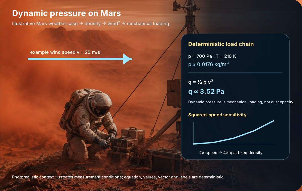
Primary-source map for this operational dossier
Mars weather operations casebook — turn atmospheric measurements into protected decisions
A Mars weather briefing is not a decorative forecast. Pressure, temperature, wind, dust and sky opacity interact with power, thermal control, visibility, communications, mechanical wear and EVA planning. This dossier trains the learner to reason from measured evidence to an operational gate without pretending that every local gust can be predicted precisely.

Pressure and temperature define the local thermodynamic state
Primary source: NASA/JPL — MEDA instrument.
Mars surface pressure is small compared with Earth and varies with elevation, season and weather. Temperature also changes strongly with time of day and local terrain. The pair must be interpreted together because density, convective heat transfer and instrument behaviour depend on the local state rather than on one average number.
A station trend becomes useful only when sensor height, calibration, sampling interval and location are known. A pressure change measured inside a disturbed flow field near equipment may not represent the surrounding atmosphere.
Boundary-layer weather is where people and machines operate
Near the surface, heating and cooling of the ground create a boundary layer with turbulence, slope flows and strong daily cycles. Regional models can be informative while still missing the exact wind at one rover or airlock. Operations therefore combine forecast context with local measurement.
The crew should learn to distinguish a synoptic trend from a local gust regime. That distinction affects whether a hazard is expected to persist across the site or is tied to one terrain feature or time of day.
Dust is a systems contaminant as well as an atmospheric variable
Airborne dust changes opacity and visibility; deposited dust changes solar output, optical performance, seals, radiators and mechanisms. Dust risk therefore has an atmospheric phase and a contamination phase. A storm can end while the engineering consequences continue.
The operational log should record both atmospheric indicators and hardware state. Cleaning a sensor can restore one reading without restoring solar-array performance, while a power decline can occur from accumulated deposition even when the sky appears clearer.
Forecast confidence must travel with the forecast
Primary source: NASA — Mars facts.
A single predicted value hides uncertainty. A useful briefing states the expected range, confidence, update time and threshold that would change the plan. If several sensors disagree, the decision should not average them blindly; investigate sensor health and spatial variability.
For EVA or rover dispatch, a low-confidence benign forecast may deserve the same caution as a moderate hazard. The question is whether the mission can tolerate being wrong and how quickly the crew can retreat if conditions evolve unfavourably.

Weather couples directly to power and thermal margins
Reduced sunlight can cut array output at the same time that low temperatures increase heater demand. Wind and dust can also alter heat transfer and radiator performance. Those couplings matter more than a weather variable in isolation.
An operations board should therefore translate atmospheric evidence into system consequences: expected generation, battery draw, heater duty, thermal state, communications margin and mobility restrictions. That is the bridge between meteorology and mission safety.
Sensor quality is part of atmospheric science
A weather station has siting, calibration, contamination and failure modes. A dust-covered optical sensor, a damaged wind transducer or a temperature sensor heated by nearby hardware can produce plausible but wrong data.
Cross-check independent channels where possible. A reported dust increase should be consistent with optical, power or imaging evidence; a pressure step should be compared with other stations or vehicle sensors. Agreement does not prove truth, but disagreement is a reason to investigate before committing to a high-consequence action.
A weather gate should be reversible when uncertainty is high
Primary source: NASA — Mars 2020 science instruments.
If conditions are marginal, operational choices can preserve options: shorten the traverse, keep a rover nearer a refuge, delay a dusty mechanism deployment or move energy-intensive work away from the expected low-generation period. These are not signs of forecasting failure; they are ways to operate safely under uncertainty.
A good gate names the trigger for escalation and the trigger for release. Without a release criterion, temporary restrictions can become indefinite habits; without an escalation criterion, crews can normalise slowly worsening conditions.
Post-event analysis improves the local climatology
Every storm, pressure anomaly or dust deposition event is an opportunity to compare forecast, observation and system response. The objective is not to prove the forecaster right but to improve the site model.
Archive the atmospheric state with engineering consequences. Over time the settlement learns which opacity values correspond to actual power losses, which winds mobilise local dust, how fast panels recover and which terrain produces recurring hazards.
Qualification casebook — six board decisions
1. Forecast is benign but local wind rises rapidly. A rover is preparing to cross exposed terrain.
Reasoned disposition — open after making your own decision
Use the local measurement for the local decision, verify sensor health and preserve retreat. Regional forecast confidence does not override direct hazardous evidence.
2. Opacity improves but solar output stays low. Panels were exposed during the storm.
Reasoned disposition — open after making your own decision
Suspect deposition or hardware effects. Treat atmospheric recovery and power-system recovery as separate gates.
3. Two pressure sensors differ by 7%. Both are within their individual operating ranges.
Reasoned disposition — open after making your own decision
Check calibration, height, placement and disturbance before averaging. The discrepancy itself is evidence that the state is not yet well constrained.
4. A low-confidence forecast predicts a strong overnight temperature drop. Battery margin is modest.
Reasoned disposition — open after making your own decision
Pre-heat or reschedule flexible loads while power is available, then update the plan as observations arrive. Protect the option to be conservative without committing to a permanent restriction.
5. A dust event begins during an EVA. Visibility is still acceptable.
Reasoned disposition — open after making your own decision
Use pre-defined retreat and power thresholds rather than waiting for visual conditions to become bad. Dust can degrade energy and mechanisms before human visibility becomes critical.
6. Repeated afternoon gusts occur only near one ridge. The base-wide forecast looks normal.
Reasoned disposition — open after making your own decision
Treat the ridge as a local micro-meteorological hazard and encode that lesson in route planning instead of generalising it to the entire site.
Mastery studio — four extended review problems
Use these weather problems to translate uncertain atmospheric evidence into reversible operational gates rather than treating a forecast as a command.
1. Dust-power compound event. Opacity rises gradually for three sols while deposited dust is also reducing panel output. Construct the operations response without double-counting or ignoring either effect.
Extended reasoned answer — open after attempting the problem
Separate atmospheric attenuation from surface deposition. Use sky-opacity measurements and independent array-performance trends to estimate how much generation loss is associated with each mechanism, while acknowledging uncertainty. Move flexible loads, protect battery reserve and define cleaning or alternate-generation actions. When the sky clears, do not automatically restore the old power forecast until array performance is verified. The event closes only when both the atmosphere and the hardware have recovered sufficiently for the planned loads.
2. Conflicting weather stations. A fixed habitat station reports weak winds while a rover ten kilometres away reports repeated strong gusts. Both sensors pass self-test.
Extended reasoned answer — open after attempting the problem
Do not average the values into a meaningless site-wide number. Compare terrain, sensor height, local time, exposure and recent calibration. The rover may be inside a slope-flow or channelised-wind regime that does not exist at the habitat. Use the local measurement to govern the local rover decision and preserve the fixed station for the habitat decision. Over time, the discrepancy becomes useful micro-meteorology rather than an instrumentation nuisance.
3. Forecast with wide uncertainty. The most likely forecast is acceptable for an EVA, but the upper tail crosses the retreat threshold. The science target is valuable but not time-critical.
Extended reasoned answer — open after attempting the problem
The decision should reflect the consequence of being wrong. A non-time-critical objective does not justify spending the entire uncertainty margin. Delay, shorten the route, stage the rover nearer a refuge or set an early turnaround trigger based on real-time observations. State what new evidence would release the restriction. This converts uncertainty into a reversible operating posture instead of pretending the central forecast is certain.
4. Cold-night thermal planning. The predicted overnight minimum is lower than usual, and heater demand may overlap with reduced solar recovery after a dusty afternoon.
Extended reasoned answer — open after attempting the problem
Translate the weather scenario into an energy timeline. Identify pre-heating opportunities, nonessential loads that can be shifted, battery reserve that must remain protected, and temperatures at which equipment enters a safe configuration. Update the plan when actual temperature and generation data arrive. The atmospheric forecast matters because it changes the power-and-thermal state; the final decision should therefore be expressed in system margins, not only degrees Celsius.
Primary sources used in this qualification dossier
Closure standard. The learner can connect atmosphere measurements to power, thermal and EVA consequences, carry forecast uncertainty into the gate and define a reversible operating response.
Forecast verification and sensor siting — build a local weather service that learns
The corrected atlas now separates vertical atmospheric structure from time evolution. The operational layer extends that discipline into operations: measurements need declared height and exposure, forecasts need uncertainty, and every forecast should eventually be compared with what actually happened. A settlement weather service becomes useful by learning its biases, not by issuing confident icons.

Sensor siting changes the weather you think you measured
A pressure sensor in a well-ventilated enclosure, a temperature sensor heated by structure, and a wind sensor in the wake of a habitat can all report real voltages while representing the local environment poorly. Metadata should therefore record sensor height, nearby obstacles, thermal exposure, calibration and maintenance history.
The goal is not to find a magically perfect site. It is to know what each site represents. A mast may sample the free flow better than a low sensor while a low sensor may better represent the conditions experienced by a rover intake or astronaut near the ground.
Vertical profiles and local-time cycles answer different questions
A vertical profile asks how a variable changes with height at a specified time or atmospheric state. A local-time series asks how a variable changes through the sol at a specified sensor height. Combining those questions on one unlabeled axis can teach a false physical relationship, which is why the current course keeps them in separate panels.
The operational payoff is clear: a morning inversion, afternoon mixing and nighttime cooling can change the relationship between a surface sensor and conditions a few metres or tens of metres above it. The team states both height and local time whenever a profile or threshold is used.
Forecasts should carry uncertainty and verification history
A forecast that says ‘wind 12 m/s’ without uncertainty hides the decision problem. Operations need the predicted distribution or at least an interval/confidence class, plus knowledge of how the local model performed under comparable conditions. The same 12 m/s forecast can justify GO or HOLD depending on the allowed threshold and forecast error.
After the event, observed conditions are compared with the forecast. Bias, missed events and false alarms are recorded. Over time this creates local verification statistics. Mars 2020 MEDA is a primary source bridge for actual Mars atmospheric measurements; Delta-Sierra’s verification loop is a pedagogical operations construct.
Dust hazard propagates through multiple systems on different timescales
Atmospheric dust can change illumination, contaminate surfaces, alter thermal behaviour, reduce imaging quality and raise maintenance workload. The effect on solar energy may persist after winds improve because deposited dust remains on panels. A weather event therefore has both atmospheric duration and system-recovery duration.
The settlement should report the state of the atmosphere and the state of affected systems separately. A forecast can end while the power system is still recovering. This prevents a premature return to full activity based on ‘weather cleared’ alone.
A local climatology is an operational asset, not merely a science archive
Repeated observations can identify seasonal patterns, site-specific wind channels, recurring pressure tides and the performance of local forecasts. The record should include sensor configuration changes so apparent climate shifts are not actually instrumentation shifts.
The module should train the learner to ask whether a threshold is based on enough relevant history. NASA Mars facts provides the broad planetary context; local operational climatology must be built from site measurements and qualified models.
Operational review board — five decisions to defend
1. Wind sensor moved after construction. Reported winds drop sharply the next week.
Reasoned disposition — open after making your own decision
Check siting and wake effects before claiming a climate change. Configuration metadata are part of the data.
2. Forecast near EVA threshold. The mean forecast is just below the limit but uncertainty overlaps unsafe conditions.
Reasoned disposition — open after making your own decision
Use the declared risk policy and reversible HOLD/shorten options instead of treating the mean as certainty.
3. Dust optical depth improves, power does not. Sky conditions recover but array output remains depressed.
Reasoned disposition — open after making your own decision
Separate atmospheric recovery from deposited-dust recovery and inspect/clean the array under its own criteria.
4. Temperature trend differs between two heights. The sensors disagree during the morning.
Reasoned disposition — open after making your own decision
Do not average blindly; investigate vertical structure, calibration and local exposure. The disagreement may be physically meaningful.
5. Forecast misses two similar events. A model repeatedly underpredicts evening gusts.
Reasoned disposition — open after making your own decision
Update local verification/bias handling and widen decision margins until performance improves.
Mission rehearsal notebook — reason through evidence before revealing the disposition
Operations drill — sensor network redesign after habitat expansion
A new berm and habitat module alter the wind field around the original mast. Rather than treating the legacy sensor as permanently authoritative, the team performs a siting review. It compares simultaneous readings from temporary reference sensors, documents wake effects and decides whether the operational climatology needs a metadata break. Historical data are not discarded; the configuration change is marked so analysts know that before/after values are not strictly homogeneous.
Operations drill — forecast skill depends on regime
The local model performs well in clear afternoon conditions but poorly during dusty evening transitions. A single overall accuracy score hides this difference. The team stratifies verification by regime and applies wider operational margins where skill is lower. This is a practical use of statistics: the question is not whether the model is ‘good’ but where it is good enough for a particular decision.
Operations drill — atmospheric recovery and hardware recovery diverge
A dust event ends and visibility improves, yet solar output, radiator performance and optical sensors remain degraded by deposition. The weather team closes the atmospheric event while operations keeps the affected hardware in a recovery state. This separation prevents a common category error: the atmosphere can return to benign conditions before the settlement has recovered from what the atmosphere did to it.
Primary sources used in this exercise
Closure review — a Mars weather service is a measurement system with a memory
The course is closed only when the learner can distinguish atmosphere from instrumentation, local weather from climatology, forecast from observation and the end of a weather event from recovery of the hardware it affected. A settlement weather service is therefore an operational chain: sensors, metadata, quality control, forecast, decision gate, verification and post-event learning.
Sensor metadata must change when the environment around the sensor changes
A mast can remain electrically healthy while a new berm, habitat or dust accumulation changes the flow around it. The record should therefore include sensor height, orientation, nearby geometry, calibration state, maintenance and configuration changes. A long time series with an undocumented siting change can look precise while mixing two different measurement environments.
Forecast skill should be conditioned on regime
One average accuracy score can hide that a model performs well on clear afternoons and poorly during dusty transitions. Verification should therefore preserve the regime, lead time and variable that mattered to the decision. The operations team can then widen margins where forecast skill is weak instead of pretending all forecasts deserve equal confidence.
Weather recovery and system recovery are separate gates
Wind can fall and visibility can improve while solar arrays, radiators, optical sensors and seals remain affected by deposition. The meteorological event can be closed while maintenance remains open. That distinction stops the phrase “the storm is over” from becoming accidental permission to resume nominal operations.
Closure case — two masts disagree after a construction change
Do not average them immediately. Compare siting, height, wake exposure, calibration and simultaneous reference measurements. If the disagreement is explained by local flow, both instruments may be correct for different micro-environments. The operational question is which environment matters to the decision.
Closure drill — separate opacity, airborne dust and deposited dust
These states affect different operations. Atmospheric opacity changes solar input and visibility; airborne particles affect sensors, seals and local flow; deposited dust can continue to degrade arrays or radiators after the atmosphere clears. A post-event review should therefore record both atmospheric recovery and hardware recovery.
Closure drill — preserve calibration and siting lineage
When a sensor is replaced, relocated or recalibrated, the metadata change becomes part of the climatic record. Analysts should know where continuity is strong and where a configuration break means that a before/after comparison needs caution.
Primary bridges: Mars 2020 MEDA and NASA Mars facts.