


Orbits: understanding free fall, energy and manoeuvres

An orbit is not a place where gravity disappears. It is continuous fall that keeps missing the surface. This module builds that intuition and connects circular speed, period, energy, vis-viva, Hohmann transfers and rendezvous. Every formula includes units and a worked check.
1. Why does a satellite not hit the ground?
It is falling. Gravity continually curves the path while tangential velocity carries the spacecraft forward. For a circular orbit, the dedicated circular-speed mini-lesson later in this course derives the relationship between gravitational parameter, centre-to-centre radius and speed. the circular-speed relationship developed in the dedicated mini-lesson.
Exercise A
The dedicated circular-speed mini-lesson later in this course uses declared Earth training values corresponding to roughly 400 km altitude and performs the conversion and unit check line by line.
The worked mini-lesson obtains about 7.67 km/s and verifies the speed unit explicitly.
Energy and angular momentum provide a second language for orbit
In the two-body problem, an orbit can be described with two ideal invariants: specific mechanical energy and specific angular momentum. Specific energy is the specific-energy relationship developed in the dedicated mini-lesson, measured in J/kg, equivalent to m²/s². Here v is speed in m/s, μ gravitational parameter in m³/s² and r distance from the central body in metres. A negative specific-energy state is bound, zero is the parabolic boundary and a positive state is hyperbolic. Specific angular momentum is built from the position and velocity vectors, has square-metres-per-second units and points perpendicular to the orbital plane. These quantities explain why a tangential burn near periapsis strongly changes apoapsis: the spacecraft changes energy where its speed is already high. They also provide independent checks when orbital elements from software look suspicious.
2. Orbital period
For a circular orbit, the orbital-period relationship developed in the dedicated mini-lesson. Using the same numbers gives about 5,545 s or 92.4 minutes.
3. Ellipses, apsides and energy
Periapsis is nearest to the central body and apoapsis farthest away. The semimajor axis a controls specific orbital energy: the bound-orbit energy/semi-major-axis relationship explained in the dedicated energy lesson for a bound Keplerian orbit. A prograde burn at periapsis raises the opposite side of the orbit; a retrograde burn lowers it.
Recover orbital period from Kepler’s third law
The dedicated orbital-period mini-lesson develops the Keplerian period relation, defines the semi-major axis and gravitational parameter, and checks units line by line. Its circular-Earth training example at a 7,000 km centre-to-centre radius produces a period of about 5,828 seconds, or 97.1 minutes. The important operational lesson is that period grows faster than radius, so a small deliberate change in semi-major axis changes timing enough to accumulate relative phase over several revolutions.
4. Vis-viva
Vis-viva — recover orbital speed from radius and orbital energy
- 1 — Concrete question
- At a known point on a two-body Keplerian orbit, what speed should the spacecraft have if its current radius and semi-major axis are known?
- 2 — Intuition without symbols
- Speed depends on both where the spacecraft is now and how much orbital energy the whole trajectory has. Falling deeper into the gravity well increases speed; belonging to a larger-energy orbit also changes the speed allowed at the same radius.
- 3 — Quantities first
- v is spacecraft speed, μ is the central body's gravitational parameter, r is current distance from the central body's centre, and a is the orbit's semi-major axis.
- 4 — Formula
- v² = μ(2/r − 1/a)
For direct evaluation of speed: v = √[μ(2/r − 1/a)]. - 5 — Read aloud
- “v squared equals mu times two over r minus one over a.” For speed, take the positive square root of that quantity.
- 6 — Symbols
- v: speed; μ: gravitational parameter; r: instantaneous central-body radius; a: semi-major axis. The square on v means v multiplied by itself.
- 7 — Pronunciation
- μ is read “mu”. The expression 1/a is read “one over a”.
- 8 — Units
- If μ is in km³/s² while r and a are in km, the bracket has units 1/km, so μ times the bracket has km²/s² and the square root gives km/s.
- 9 — Convention
- Use radius from the centre of the central body, not altitude above the surface. Keep μ, r and a in one consistent unit system and state which central body defines μ.
- 10 — Why these quantities are related
- The equation is another form of conservation of specific orbital energy: v²/2 − μ/r = −μ/(2a). The current radius sets gravitational potential while a encodes the orbit's total specific energy.
- 11 — Assumptions
- Two-body Keplerian motion with one dominant central body. The equation does not by itself include atmosphere, oblateness, third-body gravity, thrust during the evaluated point, navigation error or manoeuvre uncertainty.
- 12 — Unit check
(km³/s²) × (1/km) = km²/s², then√(km²/s²) = km/s.- 13 — Numerical case
μ = 398,600 km³/s²r = 7,000 kma = 10,000 km2/r = 2/7,000 = 0.000285714 km⁻¹1/a = 1/10,000 = 0.000100000 km⁻¹v² = 398,600 × (0.000285714 − 0.000100000) ≈ 74.0257 km²/s²v = √74.0257 ≈ 8.604 km/s- 14 — Why each operation is performed
- Compute the two inverse distances first because the equation compares the current potential term 2/r with the orbit-energy term 1/a. Multiply their difference by μ to obtain speed squared, then take the square root to recover speed.
- 15 — Algebra check
- If speed and radius are measured instead, the same equation can be rearranged as
a = 1 / (2/r − v²/μ). This is useful as a cross-check, but only when the denominator is physically consistent with the intended conic. - 16 — Mental estimate
- At 7,000 km from Earth, circular speed is about 7.55 km/s. Because this point lies below the 10,000 km semi-major axis and therefore near the faster part of the ellipse, a value moderately above circular speed—about 8.6 km/s—is plausible.
- 17 — Interpretation
- Under the stated two-body assumptions, the spacecraft should be moving about 8.60 km/s at r = 7,000 km on an orbit with a = 10,000 km.
- 18 — What the result does not prove
- It does not identify the direction of the velocity vector, guarantee a safe trajectory, prove the state estimate is correct, or replace propagation and navigation for an operational manoeuvre.
- 19 — Limit and sensitivity cases
- If a = r, vis-viva reduces to circular speed. As a tends toward infinity for the parabolic limit, it approaches escape speed
√(2μ/r). If inconsistent inputs make the term inside the square root negative for the claimed conic, stop and inspect the state, units and model instead of forcing a numerical answer. - 20 — Practice
Guided exercise. Around Earth use μ = 398,600 km³/s², r = 9,000 km and a = 12,000 km. Compute the speed.
Guided correction — open after attempting the guided exercise
Detailed guided correction.
2/r = 2/9,000 = 0.000222222 km⁻¹.1/a = 1/12,000 = 0.000083333 km⁻¹.- Difference =
0.000138889 km⁻¹. v² = 398,600 × 0.000138889 ≈ 55.3611 km²/s².v ≈ √55.3611 ≈ 7.441 km/s.
Autonomous exercise. A tracked Earth-centred state gives r = 8,000 km and speed v = 8.00 km/s. Use vis-viva to estimate the semi-major axis and state what the result still cannot tell you.
Autonomous correction — open after attempting the exercise
One defensible worked solution.
v²/μ = 64/398,600 ≈ 0.000160562 km⁻¹.2/r = 2/8,000 = 0.000250000 km⁻¹.1/a = 0.000250000 − 0.000160562 = 0.000089438 km⁻¹.a ≈ 1/0.000089438 ≈ 11,181 km.- The value describes orbital energy in the ideal model; without velocity direction and full state it does not determine orientation, exact apsides or collision/safety geometry.
- 21 — Mission decision
- Use vis-viva as an independent energy/speed cross-check. If propagated speed, reconstructed burn performance and vis-viva disagree beyond the expected uncertainty, place the next irreversible manoeuvre on HOLD until frames, units, state, manoeuvre reconstruction and model assumptions reconcile.
This relation connects position, speed and energy. For a circular orbit, the semi-major axis equals the orbital radius, so the general energy relationship reduces to the circular-speed case developed in its dedicated mini-lesson.
Exercise B
The vis-viva mini-lesson later in this course uses a declared Earth training state and walks through every numerical operation.
That worked vis-viva case produces a speed of about 8.60 km/s after the unit and order-of-magnitude checks.
Use vis-viva as a fast numerical cross-check
The dedicated vis-viva mini-lesson relates local speed to centre-to-centre radius and semi-major axis, with a strict one-unit-system rule. Its Earth training case compares a 7,000 km circular state with the periapsis of a 10,500 km transfer ellipse and obtains an ideal first impulse of roughly 1.16 km/s. The purpose of keeping that worked solution in one complete mini-lesson is to make it an auditable independent check on astrodynamics software, especially when radius-versus-altitude or unit errors are possible.
5. Hohmann transfer
A Hohmann transfer between coplanar circular orbits uses a tangent half-ellipse. One impulse enters the transfer; another circularises. It is a minimum-energy model under simplified assumptions, not a universal mission optimum when flight time, plane changes or low thrust matter.
The same geometry provides first intuition for Earth-to-Mars transfer around the Sun. Departure timing matters because Mars must reach the intercept point when the spacecraft does.
6. Rendezvous requires phase, not just orbit
Two vehicles must occupy the same place at the same time with compatible velocity. Phasing uses a temporary orbit with a different period. A common intuition trap is to “speed up toward” the target; changing speed changes the orbit and can change average angular rate in the opposite way expected.
Hohmann is a benchmark, not a universal command
A Hohmann transfer between circular coplanar orbits uses two impulses and minimises Δv within that specific model. It does not automatically minimise time, operations risk or real mission cost. A mission may spend more Δv to shorten exposure, meet lighting constraints or arrive at a required rendezvous phase. The first burn enters an ellipse whose periapsis matches the lower orbit and apoapsis the upper orbit; the second circularises. A reliable hand calculation obtains circular and transfer speeds separately with vis-viva, then forms each velocity difference. Total Δv is the sum of the absolute burn magnitudes, in m/s or km/s. Treating Hohmann as a reference case rather than a rule makes later optimisation easier to understand.
7. What two-body theory omits
Real missions add oblateness, atmosphere, third bodies, solar radiation pressure, manoeuvre errors and navigation uncertainty. The simple model remains essential for intuition and for detecting impossible numerical results before high-fidelity propagation.
Two-body theory has a clearly defined boundary
The two-body model assumes point masses and one dominant central gravity field. Real trajectories also experience oblateness, third-body gravity, atmospheric drag in low orbit, solar radiation pressure and manoeuvre errors. The correct lesson is not that the simple model is useless; it is that each omitted effect has a time and accuracy scale. A minutes-long hand calculation may be excellent for checking an impulsive transfer, while months of precise orbit prediction require perturbations and numerical integration. Model fidelity should therefore be chosen from the decision being made. Before adding complexity, quantify the error allowed in position, velocity, event time or propellant and ask whether the simpler model already meets it.
8. Check yourself
- Explain orbit as free fall.
- State the units of μ.
- Why is speed higher at periapsis?
- Why is rendezvous also a timing problem?
9. Escape speed: leave a bound orbit
The dedicated escape-speed mini-lesson below derives the two-body zero-energy boundary and shows why ideal escape speed is about 1.414 times circular speed at the same radius. Escape does not mean gravity disappears; it means the idealized two-body specific orbital energy is no longer negative.
Exercise D
The escape-speed mini-lesson below uses the same low-Earth-orbit training radius and then compares its result with circular speed.esc The resulting ideal escape speed is about 10.85 km/s; compare its scale with the previously developed circular-speed result.
10. Plane change prefers lower speed
The dedicated plane-change mini-lesson later in this course derives the instantaneous velocity-vector rotation relationship and works the 7.7 km/s, 10° training case. That case costs about 1.34 km/s, showing why launch inclination and the location of a plane change matter greatly.
Ellipse geometry and rendezvous belong in the same toolkit
For an ellipse, the semi-major axis is the arithmetic mean of periapsis and apoapsis radii; the following development uses that geometric definition without hiding it in a symbol-only line. eccentricity is a dimensionless measure of how unequal periapsis and apoapsis radii are: zero describes an ideal circle and larger values describe increasingly elongated ellipses. These parameters define geometry but not where a spacecraft is at a particular time. Rendezvous adds phase: two vehicles can have identical orbital elements and still be separated by hundreds of kilometres. A practical design therefore moves between inertial orbital elements and a relative frame near the target. Far away, transfer energy and period dominate; close in, line-of-sight rate, closing velocity and collision geometry become critical. This transition explains why “same orbit” is only a prerequisite for rendezvous, not the rendezvous solution itself.
11. Phasing: change period to change angle
If a target is ahead on the same orbit, pointing thrust directly at it is wrong. A temporary semimajor-axis change modifies orbital period, allowing relative phase to evolve before final rendezvous manoeuvres remove position and velocity differences.
Plane change exposes why geometry and timing matter
For an instantaneous plane change of angle Δi at speed v, a useful relationship is the vector plane-change relationship developed in the dedicated mini-lesson. Δv and v share the same velocity unit; Δi must be provided in the angular unit expected by the sine function, usually radians in software. The dedicated plane-change mini-lesson works the 7.5 km/s, 10-degree case and obtains about 1.31 km/s. Repeating the same angular change at 2.0 km/s costs only about 0.35 km/s. Mission designers therefore try to combine plane change with another manoeuvre where speed is low. Rendezvous adds a further constraint: matching an orbital plane or altitude is insufficient unless the vehicles also reach the same place at the same time.
Phasing changes time to change angle
Phasing exploits the connection between semi-major axis and period. A vehicle that briefly moves to a slightly lower orbit has a shorter period and advances in phase relative to a target on the original orbit; a higher phasing orbit does the opposite. The design problem is to choose a temporary period such that, after an integer or selected fraction of revolutions, the relative angle closes at the desired point. Burns then enter and leave the phasing orbit. This is not free: Δv, minimum altitude, lighting, communications and conjunction risk constrain the solution. A spreadsheet can explore candidate periods, but a final rendezvous plan also needs relative navigation and bounded closing speed.
12. Mars orbits are service geometries
Relay, crew-staging and mapping orbits optimise different goals. Altitude and inclination change coverage, period, eclipse, radiation, insertion cost and site visibility. Highly elliptical orbits can provide long dwell over a region at the price of varying range.
13. Reference frames can simplify or break the problem
An orbital state is position and velocity in a defined frame at a defined time. Inertial frames support dynamics; rotating frames can simplify relative problems; local frames support operations. Transformations require explicit conventions and time handling.
A Mars orbit is selected for the service it provides
Low Mars orbit supports close observation and can reduce some surface-link distances, but it has high orbital speed and frequent occultations. Higher orbits cover more of the planet and can support relay service at the cost of greater range and delay. Highly elliptical orbits dwell near apoapsis for long periods but pass through a wider thermal and radiation environment. The correct choice therefore starts with the service—communications, mapping, rendezvous, vehicle staging or landing support—and then evaluates periods, eclipses, line-of-sight geometry and manoeuvre cost. Orbital mechanics defines the possible paths; mission architecture chooses which path makes the required operation reliable.
14. Mini-project
Two vehicles share a circular Mars orbit and are separated by 20°. Decide qualitatively whether the chaser needs a temporarily shorter or longer period to close the phase angle. Only after explaining the direction should you use a numerical propagator.
Mini-project: close geometry, timing and Δv together
A useful mini-project starts with two circular orbits, a target phase offset and a maximum manoeuvre budget. First compute circular periods. Then choose a transfer or phasing ellipse and use vis-viva to calculate burn magnitudes. Propagate the elapsed time to determine where the target will be when the chaser arrives. If the phase does not close, change the temporary semi-major axis rather than forcing a final large correction. Record every distance as radius or altitude explicitly and keep μ units consistent. The project is complete only when geometry, time and velocity all agree. This is the same discipline later required by numerical rendezvous tools: a trajectory is not valid because one Δv number looks plausible.
15. Energy tells you whether the path is bound
Specific orbital energy the specific-energy relationship developed in the dedicated mini-lesson is negative for an ellipse, zero for ideal escape and positive for a hyperbola. This single equation lets you classify a trajectory before calculating every orbital element. It is especially useful after a partial burn: engine status alone does not tell whether capture succeeded.
16. Why burns at periapsis are powerful
Because speed is highest near periapsis, a given prograde Δv there produces a large energy change. This is the intuition behind the Oberth effect. The effect does not create energy for free; the engine adds the same velocity increment, but performing it where the spacecraft already moves rapidly changes kinetic energy more strongly.
17. Plane change and rendezvous compete for Δv
A mission designer tries to combine manoeuvres when geometry permits, because a separate large plane change can be expensive. Rendezvous planning therefore begins with launch plane, phasing and arrival geometry, not only with the final close approach.
Plane change and rendezvous compete for the same budget
A mission rarely has separate propellant tanks labelled “plane change” and “rendezvous.” All manoeuvres consume the same Δv reserve. If the target orbit differs in inclination, performing the plane change where speed is lower can save substantial propellant, but the resulting geometry may complicate phasing or communications. Combining a plane change with another burn can reduce total vector change when the directions are chosen correctly. The trade is therefore multi-dimensional: total Δv, time, eclipse, navigation observability and operational complexity. A good design records not only the mathematically minimum manoeuvre but a robust sequence that can tolerate injection error and still preserve collision-avoidance authority.
18. Numerical-tool readiness check
Before using an orbit propagator, write down central body, μ, frame, epoch, position and velocity units. Then predict qualitatively what the trajectory should do. If the software produces a result with the opposite trend, investigate the inputs before trusting the plot.
Engineering studio — reconstruct an orbital manoeuvre
The scenario starts from a circular Mars orbit near 3,800 km from the planet centre and targets an orbit whose apoapsis reaches 6,000 km. Reuse the complete vis-viva mini-lesson rather than introducing a second compressed equation: compute speed before and after the impulse with one consistent unit system, then explain why an impulse near periapsis mainly raises apoapsis. The task is to transfer a method, not memorize a final number.
Now add a +1 m/s execution error. The student estimates its consequence for apoapsis and selects a correction policy: correct at once, wait for better observability, or retain the error if the orbit remains inside the accepted envelope. The choice depends on Δv cost, time, navigation accuracy, collision risk and eclipse geometry. Orbital mechanics therefore becomes an operational decision rather than a formula exercise.
Worked comparison — plane change now or after raising apoapsis?
For an instantaneous plane change of angle Δi at speed v, the required velocity change is the vector plane-change relationship developed in the dedicated mini-lesson. The same angular change therefore costs less where orbital speed is lower. Compare a 10° plane change at 7.7 km/s with the same change at 3.0 km/s: the geometry is identical, but the velocity penalty is not. This is why mission designers often combine plane changes with burns near apoapsis or other low-speed points.
The comparison also shows a trap: raising apoapsis costs Δv too. A good solution adds the burn used to reshape the orbit, the cheaper plane change and any burn needed to restore the final orbit. “Do it where speed is low” is a useful principle, but the complete manoeuvre sequence decides whether the strategy actually saves propellant.
First Man orbital mechanics dossier — close geometry, timing and delta-v
Orbital mechanics becomes operational when the learner can define a state, select the central body and reference frame, calculate a manoeuvre, propagate the resulting orbit, and explain what the manoeuvre buys in mission terms. A correct equation with the wrong radius, epoch or frame is not a correct solution.
State comes before manoeuvre
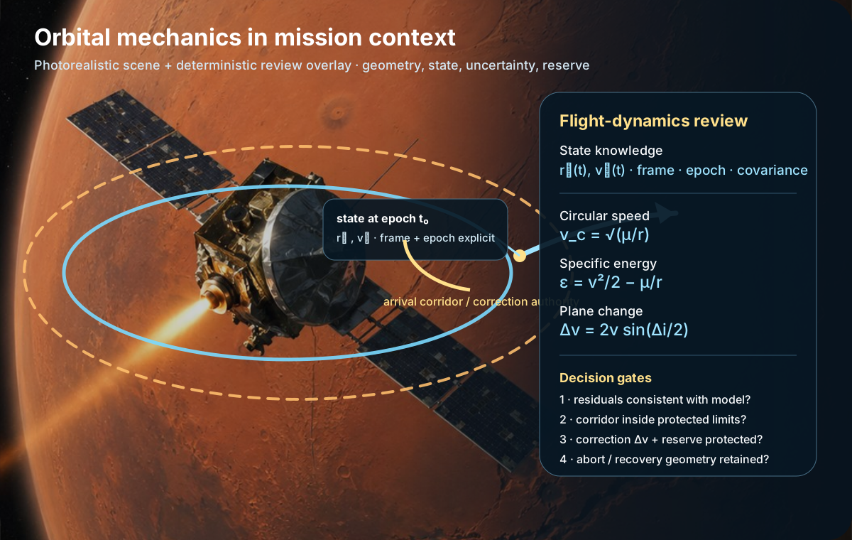
A spacecraft state contains position and velocity at an epoch in a defined frame. The JPL Solar System Dynamics — Orbits and ephemerides is a primary reference for orbit and ephemeris concepts. Before calculating a burn, write the central body, coordinate frame, epoch, position or orbital elements and current velocity. Without those, ‘raise the orbit’ is an incomplete instruction.
Altitude is not radius. Orbital equations normally use distance from the centre of the body. Around Earth, a 400 km altitude corresponds to a radius of roughly Earth radius plus 400 km. Confusing those values produces a severe speed error while leaving the algebra looking clean.
Energy, angular momentum and geometry are complementary checks
Two-body orbital motion can be described with several equivalent languages. Energy tells whether a trajectory is bound and how semi-major axis changes; angular momentum helps explain geometry and plane; conic elements describe the orbit shape and orientation. NASA Science — Gravity and mechanics provides a foundation for gravity and mechanics.
When a numerical propagator produces a surprising answer, these invariants become diagnostic tools. A prograde burn near periapsis should usually raise the opposite side of an ellipse. If software reports the opposite without a frame or sign explanation, investigate before accepting the plot.

Hohmann transfer is a benchmark, not a universal command
The two-impulse Hohmann transfer between coplanar circular orbits is valuable because it gives an analytically clean benchmark. It does not automatically minimize elapsed time, operational complexity or total mission risk. Plane changes, finite burn duration, perturbations, launch windows and rendezvous constraints can make another strategy preferable.
The JPL — Fundamentals of Orbital Mechanics provides a deeper orbital-mechanics reference. A student should be able to derive or reproduce the benchmark, then state which assumptions would have to be relaxed for a real mission design.
Timing is part of geometry
Rendezvous is not solved by reaching the same orbit. The chaser and target must reach the same place at the same time with compatible relative velocity. Phasing deliberately changes orbital period so relative angle accumulates. The sign of the period change determines whether the chaser gains or loses phase.
For interplanetary transfers, departure time plays the same role at a larger scale. The target planet must arrive at the intercept region when the spacecraft does. A transfer calculation therefore has geometry, dynamics and calendar dimensions.

Delta-v is an inventory with uncertainty and ownership
A mission delta-v budget should separate deterministic manoeuvres from dispersions, correction allowances, attitude-control demand and protected reserve. Treating every kilogram of propellant as freely spendable creates late-mission traps. Each manoeuvre should identify which budget line it consumes and what decision gate protects the remaining reserve.
Orbital modelling conventions become increasingly important as fidelity grows; NASA Science — Planetary orbits provides additional planetary-orbit context. The training goal is not to reproduce a full flight-dynamics system by hand, but to understand enough to challenge inputs, units, frames and outputs.
Worked transfer dossier — close both burns, flight time and reserve
For the teaching transfer from a 7,000 km circular Earth-centred radius to 14,000 km, the first ideal Hohmann burn is about 1.167 km/s. The second burn is not optional: at transfer apoapsis, the spacecraft is moving more slowly than the circular speed of the higher orbit, so another prograde burn is required to circularize. Using the same two-body model, the second ideal burn is about 0.979 km/s, giving roughly 2.147 km/s total before any plane change, navigation correction, finite-burn loss or protected reserve.
The transfer ellipse in this training case has a 10,500 km semi-major axis, obtained as the mean of the two declared circular radii. Reuse the complete orbital-period mini-lesson to obtain the ellipse period and then take half of that period for the ideal coast. This gives the operator a timing expectation that can be compared with propagation software. If the tool predicts a radically different transfer time, check units, radii, central body and whether the software model describes the same manoeuvre.
The review package should show the initial orbit, transfer ellipse, final orbit, both burn vectors, transfer time and residual reserve. It should also state whether the burns are impulsive approximations. For low-thrust propulsion, the geometry and timing change enough that the Hohmann solution becomes a benchmark rather than an execution plan.
Rendezvous case — why matching altitude is not enough
A chaser and target can occupy the same circular orbit while remaining hundreds of kilometres apart. To rendezvous, the chaser deliberately changes its orbital period so the relative phase evolves. If it enters a slightly lower orbit, it moves around the central body faster and gains phase; if it enters a higher orbit, it moves more slowly and loses phase. The sign must be reasoned from orbital period, not from the intuition that ‘speeding up means go to a higher orbit’.
Near the intercept, the objective changes from shaping absolute orbit to controlling relative motion. Closing distance while leaving excessive relative velocity can create a collision. The flight dynamics plan therefore includes approach gates, hold points, sensor requirements and abort trajectories. A hand calculation cannot replace the operational procedure, but it can tell the learner whether the commanded relative trend makes sense.
| Review layer | Hand calculation | Operational evidence |
|---|---|---|
| Transfer | Δv₁, Δv₂, time of flight | Propagated state and burn solution |
| Plane | Vector-change estimate | Attitude / burn geometry |
| Phasing | Period difference | Relative-angle prediction |
| Final approach | Relative speed order of magnitude | Navigation solution, corridor, abort path |
Review drills — move from explanation to operational judgement
- Radius drill. Convert an altitude to central-body radius before using a circular-speed equation.
- Frame drill. State frame and epoch for a rendezvous state vector.
- Budget drill. Separate deterministic burn, correction allowance and protected reserve.
- Model-limit drill. List four effects omitted by the two-body Hohmann model and state which could matter most in low orbit.
First burn of an ideal Hohmann transfer
- 1 — Concrete question
- What ideal instantaneous prograde velocity change moves a spacecraft from a lower circular orbit into the transfer ellipse toward a higher circular orbit?
- 2 — Intuition without symbols
- Start with circular speed in the lower orbit, calculate how much faster the spacecraft must move at the transfer ellipse periapsis, and take the difference.
- 3 — Quantities first
- μ is gravitational parameter of the central body; r₁ lower-orbit radius; r₂ higher-orbit radius; Δv₁ first-burn magnitude.
- 4 — Formula
- Δv₁ = √(μ/r₁) × [√(2r₂/(r₁+r₂)) − 1]
- 5 — Read aloud
- “Delta-v one equals square root of mu over r one, times the square root of two r two over r one plus r two, minus one.”
- 6 — Symbols
- Δ means change; v is speed; μ is gravitational parameter; r₁ and r₂ are distances from the central body centre.
- 7 — Pronunciation
- μ is read “mu”; Δ is read “delta”.
- 8 — Units
- If μ is km³/s² and radii are km, √(μ/r) gives km/s, so Δv is km/s.
- 9 — Convention
- Use radii from the centre, not altitudes, and use one consistent unit system.
- 10 — Why this operation
- √(μ/r₁) is lower circular speed; the bracket is the ratio between transfer-periapsis speed and that circular speed.
- 11 — Assumptions
- Two-body gravity, circular coplanar initial and final orbits, instantaneous burns and no losses or perturbations.
- 12 — Unit check
- √[(km³/s²)/km] = √(km²/s²) = km/s; the bracket is dimensionless.
- 13 — Numerical case
μ = 398,600 km³/s².r₁ = 7,000 km; r₂ = 14,000 km.Circular speed factor √(μ/r₁) = √(398,600/7,000) ≈ 7.546 km/s.Geometry ratio = 2r₂/(r₁+r₂) = 28,000/21,000 = 1.3333.Square root of geometry ratio ≈ 1.1547.Bracket = 1.1547 − 1 = 0.1547.Δv₁ ≈ 7.546 × 0.1547 = 1.167 km/s.- 14 — Why each operation
- The nested roots come from orbital-energy relationships; subtracting one converts the transfer-speed ratio into an increment above circular speed.
- 15 — Algebra check
- The formula is normally evaluated directly; rearranging for r₂ is possible but not the preferred beginner workflow.
- 16 — Mental estimate
- The burn is a fraction of the roughly 7.5 km/s circular speed, so about 1 km/s is plausible; 10 km/s would be an obvious warning.
- 17 — Interpretation
- In the ideal two-body model, the first burn is about 1.17 km/s prograde.
- 18 — What it does not prove
- It does not include the second burn, plane change, finite-thrust losses, launch constraints, navigation error or propellant reserve.
- 19 — Sensitivity or limit case
- As r₂ grows, the first-burn requirement increases but does not scale linearly with altitude because orbital energy depends nonlinearly on radius.
- 20 — Practice
Guided exercise. Using the same μ and r₁ = 7,000 km, compute Δv₁ for r₂ = 10,500 km.
Guided correction — open after attempting the guided exercise
Detailed guided correction.
- Geometry ratio = 21,000/(17,500) = 1.2.
- √1.2 ≈ 1.09545; bracket ≈ 0.09545.
- Circular speed factor remains ≈ 7.546 km/s.
- Δv₁ ≈ 7.546 × 0.09545 ≈ 0.720 km/s.
Autonomous exercise. Compare two strategies conceptually: perform a 10° plane change in the original low orbit or raise apoapsis first and perform the change where speed is lower. Explain what additional calculations are required before choosing.
Autonomous correction — open after attempting the exercise
One defensible worked solution.
- Plane-change cost depends on local speed: Δv = 2v sin(Δi/2).
- Raising apoapsis costs transfer Δv but lowers speed near apoapsis.
- Compute the transfer burns plus the low-speed plane change and compare with direct plane change.
- Then include timing, operational complexity, reserve and rendezvous consequences before making the mission decision.
- 21 — Mission decision
- Use the benchmark to challenge a mission design, then protect delta-v reserve and switch to higher-fidelity modelling when the assumptions no longer match the operation.
Final astrodynamics review — challenge the trajectory before trusting the plot
- Are central body, frame and epoch explicit?
- Are all orbital distances radii from the centre when required?
- Does the hand calculation reproduce the expected order of magnitude?
- Are both burns and transfer time closed for a transfer benchmark?
- Is plane change treated as a vector operation at the actual local speed?
- Is protected delta-v reserve separate from deterministic manoeuvres?
A mission-design tool should make the analysis faster, not opaque. The learner should be able to explain what the software input means physically, predict the qualitative direction of the result and identify which model limitations require higher fidelity. A trajectory that cannot be challenged by simple physics is not ready for approval.
Primary sources used in this section
- NASA Science — Gravity and mechanics
- NASA Science — Planetary orbits
- JPL — Fundamentals of Orbital Mechanics
- JPL Solar System Dynamics — Orbits and ephemerides
Closure rule. An orbital solution is reviewable only when frame, epoch, radii, manoeuvre geometry, timing and protected delta-v reserve are all explicit.
Orbital mechanics operations laboratory — geometry, timing and energy together
This operational extension connects orbital equations to state knowledge, uncertainty, manoeuvre reconstruction, rendezvous geometry and decision gates so the learner can defend a trajectory rather than merely quote a nominal answer.
Describe the state before describing the manoeuvre
An orbit is not identified by altitude alone. Position and velocity, or an equivalent set of orbital elements, define the state relative to a chosen central body and reference frame. Before planning a burn, state the current orbit, target orbit, epoch and frame. This prevents common errors such as comparing velocities expressed in different frames or assuming that two spacecraft at the same altitude are ready to rendezvous.
Read vis-viva as an energy statement
The vis-viva relation connects orbital speed to distance from the central body and orbital energy. Its operational value is qualitative as well as numerical: speed is higher near periapsis and lower near apoapsis on an ellipse, so the same small change in velocity can have very different consequences depending on where it is applied. This is the basis for understanding why burn location matters before memorizing named manoeuvres.
Close a transfer with both burns and time of flight
A Hohmann-style transfer is not just one delta-v number. It contains a departure impulse, coast phase and arrival impulse, each defined by the initial and final circular radii under ideal two-body assumptions. The coast time affects phasing and operations. If the target spacecraft or planet is not at the right angular position at arrival, a perfectly calculated transfer ellipse still misses the mission. Geometry and timing must therefore be solved together.
Treat plane change as a vector problem
Changing orbital plane rotates the velocity vector and can be expensive when speed is high. Performing a required plane change where orbital speed is lower can reduce delta-v, but reaching that location may require other manoeuvres and extra time. The correct comparison is a complete manoeuvre sequence, not the plane-change equation in isolation. Operational constraints such as communications, lighting and navigation may also rule out the mathematically cheapest option.
Rendezvous is controlled relative motion
Two vehicles on nearly the same orbit can still separate because their orbital periods differ. Phasing deliberately changes period to change relative angle. Close rendezvous then becomes a guidance and navigation problem in which range, range rate and line-of-sight behaviour matter. A safe plan includes hold points and abort options because a late correction near another spacecraft can turn a small navigation error into a collision hazard.
Know where the two-body model stops being enough
Two-body equations are a foundation, not the whole mission. Atmospheric drag, non-spherical gravity, third-body perturbations, finite burn duration, navigation error and operational constraints can all matter. The learner should use the simple model to build intuition and independent checks, then know when a higher-fidelity tool is required. A numerical result becomes credible only when the model fidelity matches the decision being made.
Connect Mars orbit to the service it must provide
A communications relay, mapping spacecraft, crew staging vehicle and aerobraking mission may prefer different orbit geometries. Inclination, periapsis altitude, apoapsis altitude, period and line-of-sight coverage are design variables tied to a service. There is no universally 'best Mars orbit'. A mission review should therefore begin with the service requirement and derive the orbit, rather than selecting an orbit because it is familiar.
Protect delta-v with margins and decision gates
A manoeuvre budget should distinguish deterministic delta-v, navigation correction allowance, dispersion correction, attitude-control demand and protected reserve. Spending reserve early may be acceptable only if the later mission can still close under the agreed failure cases. This turns delta-v from a single mission-total number into a managed inventory with ownership and release rules.
Progressive mastery drills — eight linked checks
Drill 1 — Orbital state
List the information needed to distinguish two spacecraft that share altitude but not the same orbit.
Expected reasoning for “Drill 1 — Orbital state”: explain the physical meaning, units or evidence path, state at least one assumption, and say which operational decision would change if the result or evidence were different.
Drill 2 — Circular-orbit intuition
Explain qualitatively why lower circular orbits have higher speed around the same central body.
Expected reasoning for “Drill 2 — Circular-orbit intuition”: explain the physical meaning, units or evidence path, state at least one assumption, and say which operational decision would change if the result or evidence were different.
Drill 3 — Transfer sequence
Describe departure burn, coast and arrival burn as one timed sequence rather than one delta-v value.
Expected reasoning for “Drill 3 — Transfer sequence”: explain the physical meaning, units or evidence path, state at least one assumption, and say which operational decision would change if the result or evidence were different.
Drill 4 — Rendezvous
Explain why matching position without matching velocity is not a safe rendezvous condition.
Expected reasoning for “Drill 4 — Rendezvous”: explain the physical meaning, units or evidence path, state at least one assumption, and say which operational decision would change if the result or evidence were different.
Drill 5 — Escape condition
Use the idea of specific orbital energy to explain the boundary between a bound and unbound trajectory.
Expected reasoning for “Drill 5 — Escape condition”: explain the physical meaning, units or evidence path, state at least one assumption, and say which operational decision would change if the result or evidence were different.
Drill 6 — Plane change
Explain why plane change is generally cheaper where orbital speed is lower, while noting the cost of reaching that point.
Expected reasoning for “Drill 6 — Plane change”: explain the physical meaning, units or evidence path, state at least one assumption, and say which operational decision would change if the result or evidence were different.
Drill 7 — Phasing
Describe how a temporary change in orbital period changes relative angle to a target.
Expected reasoning for “Drill 7 — Phasing”: explain the physical meaning, units or evidence path, state at least one assumption, and say which operational decision would change if the result or evidence were different.
Drill 8 — Model fidelity
List at least four effects ignored by a simple two-body impulsive model that can matter in mission design.
Expected reasoning for “Drill 8 — Model fidelity”: explain the physical meaning, units or evidence path, state at least one assumption, and say which operational decision would change if the result or evidence were different.
Integrated exercise — Compare two plane-change strategies qualitatively
A spacecraft needs a plane change but can either perform it immediately in a low circular orbit or first raise apoapsis, perform most of the plane change near the slower apoapsis, then complete the transfer. Describe the calculations and operational factors required to decide between the strategies. Do not assume the second option is automatically better.
Reasoned solution. Compare the full delta-v of every burn, not just the plane-change component; include transfer time, navigation uncertainty, propulsion constraints, communications, thermal and lighting conditions, and the consequences of a failed or partial burn. The high-apoapsis plane change can reduce the vector-rotation cost because speed is lower there, but the extra transfer burns and operational exposure can offset that benefit.
Primary sources for this section. NASA — Basics of Space Flight: orbital mechanics NASA — Basics of Space Flight: interplanetary trajectories NASA Glenn — Flight to orbit. Use these references to verify the assumptions, limits and values that apply to the mission context.
Core orbital equations — four formula mini-lessons for zero-prerequisite mastery
These four equations already appear conceptually throughout the course. This section closes the pedagogical gap by giving each one the same full explanation contract as vis-viva and the Hohmann calculation: meaning, units, assumptions, arithmetic, limits, exercises and mission consequences.
Circular orbital speed — distinguish radius from altitude
- 1 — Concrete question
- At a given radius in an ideal circular orbit, what speed keeps the spacecraft continuously falling around the central body?
- 2 — Intuition without symbols
- Gravity bends the path inward while forward motion carries the spacecraft sideways. A circular orbit occurs when those effects match at one radius.
- 3 — Quantities first
- v_c is circular speed, μ is the central body gravitational parameter and r is distance from the body centre.
- 4 — Formula
v_c = √(μ/r)- 5 — Read aloud
- “v sub c equals the square root of mu divided by r.”
- 6 — Symbols
- v_c is circular speed; μ (“mu”) packages the body’s gravitational strength; r is centre-to-spacecraft radius.
- 7 — Pronunciation
- μ is read “mu”. The radical sign means square root.
- 8 — Units
- If μ is km³/s² and r is km, μ/r is km²/s²; the square root gives km/s.
- 9 — Convention
- Use radius from the centre, not altitude above the surface. Keep μ and r in a consistent unit system.
- 10 — Why this operation
- Circular centripetal acceleration and gravitational acceleration are set equal; solving for speed gives the square-root relationship.
- 11 — Assumptions
- Two-body gravity, circular orbit, instantaneous state and no atmosphere/thrust/third-body perturbation in the teaching model.
- 12 — Unit check
- km³/s² divided by km gives km²/s²; square root gives km/s.
- 13 — Numerical case
μ_Earth = 398,600 km³/s².r = 7,000 km.μ/r = 398,600 / 7,000 = 56.9429 km²/s².v_c = √56.9429 ≈ 7.546 km/s.- 14 — Why each operation
- Divide the gravitational parameter by radius to obtain the squared-speed scale, then take the square root because the force balance contains speed squared.
- 15 — Algebra check
- Rearranging gives
r = μ/v_c²; substituting the result recovers about 7,000 km. - 16 — Mental estimate
- Four hundred thousand divided by seven thousand is a little under 60; √60 is a little under 8, so 7.55 km/s is plausible.
- 17 — Interpretation
- A circular orbit at 7,000 km Earth-centred radius requires about 7.55 km/s in the ideal two-body model.
- 18 — What it does not prove
- It does not give escape speed, transfer-burn size, period, rendezvous phase or finite-burn effects.
- 19 — Sensitivity or limit case
- Larger radius lowers circular speed as the inverse square root. Halving radius in the mathematical model raises speed by √2, although a physical body surface may make such a radius impossible.
- 20 — Practice
Guided exercise. Compute circular speed at r = 14,000 km around Earth with the same μ.
Guided correction — open after attempting the guided exercise
Detailed guided correction.
- μ/r = 398,600/14,000 ≈ 28.471 km²/s².
- √28.471 ≈ 5.336 km/s.
- The higher circular orbit is slower, not faster.
Autonomous exercise. A tool reports 7.55 km/s for a radius entered as 7,000 m around Earth. Diagnose the error before recomputing.
Autonomous correction — open after attempting the exercise
One defensible worked solution.
- The value is plausible for 7,000 km, not 7,000 m.
- The entered radius is inside Earth and the unit is inconsistent with μ in km³/s².
- Correct the radius/unit system before trusting any result.
- 21 — Mission decision
- Use circular speed as a sanity-check baseline. If software output differs greatly, verify radius-versus-altitude, central body, frame and units before proceeding.
Orbital period — connect semi-major axis to mission timing
- 1 — Concrete question
- How long does one ideal Keplerian revolution take for a known semi-major axis?
- 2 — Intuition without symbols
- Larger orbits are longer and move more slowly, so period grows faster than orbital size itself.
- 3 — Quantities first
- T is orbital period, a is semi-major axis and μ is the central body gravitational parameter.
- 4 — Formula
T = 2π √(a³/μ)- 5 — Read aloud
- “T equals two pi times the square root of a cubed divided by mu.”
- 6 — Symbols
- T is time for one revolution; a is semi-major axis; π is pi; μ is gravitational parameter.
- 7 — Pronunciation
- π is read “pi”; μ is “mu”; a³ is “a cubed”.
- 8 — Units
- a³/μ gives seconds squared when a and μ use matching length units; the square root gives seconds.
- 9 — Convention
- For a circular orbit a equals radius. For an ellipse, a is half the major axis, not periapsis or apoapsis alone.
- 10 — Why this operation
- Kepler’s third law links period squared to semi-major axis cubed for a two-body orbit.
- 11 — Assumptions
- Keplerian two-body orbit with constant μ; perturbations and finite thrust are ignored in this hand-check.
- 12 — Unit check
- km³ divided by km³/s² gives s²; square root gives s; 2π is dimensionless.
- 13 — Numerical case
a = 7,000 km.a³ = 343,000,000,000 km³.a³/μ ≈ 860,010 s².√(a³/μ) ≈ 927.37 s.T = 2π × 927.37 ≈ 5,827 s ≈ 97.1 min.- 14 — Why each operation
- Cube the orbital size, divide by gravitational strength, take the square root to recover time, then multiply by the full-circle factor 2π.
- 15 — Algebra check
- Solving for a gives
a = [μ(T/2π)²]^(1/3). - 16 — Mental estimate
- A low Earth orbit should be on the order of one and a half hours, so about 97 minutes is reasonable.
- 17 — Interpretation
- At a 7,000 km semi-major axis, one ideal revolution takes about 97 minutes.
- 18 — What it does not prove
- It does not specify spacecraft position at an arbitrary epoch, rendezvous phase, eclipse duration or ground-track geometry.
- 19 — Sensitivity or limit case
- Period scales as a^(3/2). Doubling a multiplies T by 2^(3/2) ≈ 2.83, not by two.
- 20 — Practice
Guided exercise. Estimate the period at a = 14,000 km.
Guided correction — open after attempting the guided exercise
Detailed guided correction.
- The ratio of semi-major axes is 2.
- Period ratio is 2^(3/2) ≈ 2.828.
- T ≈ 97.1 × 2.828 ≈ 274.7 min.
Autonomous exercise. A rendezvous plan assumes that raising semi-major axis makes the chaser advance faster in phase. Explain the sign error.
Autonomous correction — open after attempting the exercise
One defensible worked solution.
- A higher semi-major axis gives a longer period.
- The higher vehicle falls behind in mean angular motion relative to a target on the lower orbit.
- A lower phasing orbit has the shorter period and advances in phase.
- 21 — Mission decision
- Use period as a fast phasing and propagation check. A trajectory timeline that disagrees strongly with the hand estimate deserves a units/model review.
Specific orbital energy — classify the trajectory before trusting the plot
- 1 — Concrete question
- Is the current ideal trajectory bound, at escape threshold or hyperbolic?
- 2 — Intuition without symbols
- Specific orbital energy compares kinetic energy per unit mass with gravitational potential energy per unit mass.
- 3 — Quantities first
- ε is specific mechanical energy, v is speed, μ gravitational parameter and r centre-to-spacecraft radius.
- 4 — Formula
ε = v²/2 − μ/r- 5 — Read aloud
- “epsilon equals v squared over two minus mu divided by r.”
- 6 — Symbols
- ε (“epsilon”) is energy per unit mass; v is speed; μ is gravitational parameter; r is radius.
- 7 — Pronunciation
- ε is read “epsilon”; μ is “mu”.
- 8 — Units
- Both terms are velocity squared: km²/s² or equivalently MJ/kg after appropriate conversion.
- 9 — Convention
- The zero-energy reference is the ideal two-body escape threshold. Keep position and speed from the same epoch/frame.
- 10 — Why this operation
- Kinetic contribution is positive; gravitational potential contribution is negative. Their sum classifies the conic.
- 11 — Assumptions
- Two-body gravity and instantaneous state; other bodies, atmosphere and active thrust are excluded.
- 12 — Unit check
- v²/2 and μ/r have identical units, so subtraction is dimensionally valid.
- 13 — Numerical case
r = 7,000 km.v = 7.546 km/s.v²/2 ≈ 28.471 km²/s².μ/r ≈ 56.943 km²/s².ε ≈ 28.471 − 56.943 = −28.472 km²/s².- 14 — Why each operation
- Square speed and halve it for kinetic energy per unit mass; divide μ by radius for gravitational magnitude; subtract because gravitational potential is negative.
- 15 — Algebra check
- For a bound Keplerian ellipse,
ε = −μ/(2a). With a = 7,000 km the same value is recovered. - 16 — Mental estimate
- Circular-orbit kinetic energy is half the magnitude of the gravitational term, so total energy should be negative with about half that magnitude.
- 17 — Interpretation
- The negative result confirms a bound orbit in the ideal model.
- 18 — What it does not prove
- A negative energy value does not guarantee collision-free geometry, stable operations, acceptable periapsis or successful capture under finite burn errors.
- 19 — Sensitivity or limit case
- At ε = 0 the trajectory is the parabolic escape limit; positive ε corresponds to a hyperbolic excess state.
- 20 — Practice
Guided exercise. Using r = 7,000 km and v = 8.60 km/s, estimate ε.
Guided correction — open after attempting the guided exercise
Detailed guided correction.
- v²/2 ≈ 36.98 km²/s².
- μ/r ≈ 56.94 km²/s².
- ε ≈ −19.96 km²/s², still bound.
Autonomous exercise. A post-burn solution reports ε > 0 although the mission intended capture. State the first three checks.
Autonomous correction — open after attempting the exercise
One defensible worked solution.
- Verify speed and position use the same frame and epoch.
- Verify radius versus altitude and μ units.
- If inputs are correct, treat positive ε as evidence that ideal capture was not achieved and evaluate correction/escape consequences.
- 21 — Mission decision
- Use specific energy as an independent capture/escape sanity check after burns. Do not infer capture from engine status alone.
Plane change — make the vector geometry and speed penalty explicit
- 1 — Concrete question
- How much ideal instantaneous Δv is required to rotate the velocity vector by a known angle without changing its magnitude?
- 2 — Intuition without symbols
- A plane change is a vector rotation. The faster the spacecraft is moving, the larger the velocity-vector tip must move for the same angular turn.
- 3 — Quantities first
- Δv is manoeuvre magnitude, v is speed at the manoeuvre and Δi is the plane-change angle.
- 4 — Formula
Δv = 2 v sin(Δi/2)- 5 — Read aloud
- “delta vee equals two vee times sine of delta i over two.”
- 6 — Symbols
- Δ means change; v is speed; i denotes inclination-like plane angle in this teaching case.
- 7 — Pronunciation
- Δ is “delta”; Δi is “delta eye”.
- 8 — Units
- The sine term is dimensionless, so Δv has the same velocity unit as v.
- 9 — Convention
- Software trigonometric functions usually expect radians. The formula assumes an instantaneous pure rotation at constant speed.
- 10 — Why this operation
- The initial and final velocity vectors form two equal sides of a triangle; the chord between their tips is the required Δv.
- 11 — Assumptions
- Instantaneous manoeuvre, same speed before and after, no simultaneous energy-changing component and no finite-burn/steering losses.
- 12 — Unit check
- 2 and sine are dimensionless; velocity times a dimensionless factor remains velocity.
- 13 — Numerical case
v = 7.5 km/s.Δi = 10°.Δi/2 = 5°.sin(5°) ≈ 0.08716.Δv = 2 × 7.5 × 0.08716 ≈ 1.307 km/s.- 14 — Why each operation
- Halve the angle because the vector triangle is symmetric; take the sine to obtain half the chord; multiply by twice the speed.
- 15 — Algebra check
- For small angles in radians, sin(Δi/2) ≈ Δi/2, so Δv ≈ vΔi. Ten degrees is 0.1745 rad; 7.5×0.1745 ≈ 1.31 km/s.
- 16 — Mental estimate
- Ten degrees is about 0.175 rad. Multiplying that by 7.5 gives roughly 1.3 km/s, matching the exact expression.
- 17 — Interpretation
- A 10° plane change at 7.5 km/s is very expensive: about 1.31 km/s ideal Δv.
- 18 — What it does not prove
- It does not say when the plane change is geometrically possible or whether raising apoapsis first reduces total mission Δv after all extra burns.
- 19 — Sensitivity or limit case
- At lower speed the same angle costs less. At zero angle the cost is zero; at 180° the formula gives twice the speed.
- 20 — Practice
Guided exercise. Compute a 10° change at v = 3.0 km/s.
Guided correction — open after attempting the guided exercise
Detailed guided correction.
- Δi/2 = 5°; sin 5° ≈ 0.08716.
- Δv = 2 × 3.0 × 0.08716 ≈ 0.523 km/s.
- The same geometry costs much less at the lower speed.
Autonomous exercise. A proposal raises apoapsis solely to perform a cheaper plane change. Explain what must be added before claiming a net saving.
Autonomous correction — open after attempting the exercise
One defensible worked solution.
- Include the burn that raises apoapsis.
- Include the burn(s) needed to restore the final orbit.
- Include timing, eclipse, navigation and operational constraints; compare total sequence Δv, not only the plane-change term.
- 21 — Mission decision
- Treat plane change as a whole-sequence vector trade. Protect collision geometry, timing and correction reserve rather than optimizing one burn in isolation.
Mission-design calculation extension — departure and arrival energy
These two mini-lessons convert hyperbolic excess speed into characteristic launch energy and propagate arrival v-infinity into a two-body local approach speed, making the handoff from trajectory design to launcher and EDL trades explicit.
Characteristic energy C3 from hyperbolic excess speed
- 1 — Concrete question
For Characteristic energy C3 from hyperbolic excess speed, how does
C3 = v_inf^2inform linking departure geometry to the launch-energy parameter used in interplanetary mission design and the operational choice “Use C3 to connect trajectory choice to launch-vehicle capability without confusing it with spacecraft propellant load.”?- 2 — Intuition without symbols
Intuition. A launcher departure can be described by how much speed remains after escaping Earth locally. Squaring that excess speed gives mission designers a compact way to compare how demanding different departures are without confusing launcher performance with the later heliocentric coast.
- 3 — Quantities first
- v_inf is hyperbolic excess speed relative to the departure planet; C3 is its square and carries speed-squared units.
- 4 — Formula
- C3 = v_inf^2
- 5 — Read aloud
- “C three equals v infinity squared.”
- 6 — Symbols
Symbol map for Characteristic energy C3 from hyperbolic excess speed. v_inf is hyperbolic excess speed relative to the departure planet; C3 is its square and carries speed-squared units.
- 7 — Pronunciation
Pronunciation. Say
C3 = v_inf^2. For Characteristic energy C3 from hyperbolic excess speed, use the step-three names tied to linking departure geometry to the launch-energy parameter used in interplanetary mission design. Speak each Characteristic energy C3 from hyperbolic excess speed unit with the quantity it measures.- 8 — Units
- (km/s)² = km²/s²
- 9 — Convention
Convention. For Characteristic energy C3 from hyperbolic excess speed, keep linking departure geometry to the launch-energy parameter used in interplanetary mission design on one declared boundary. Apply
C3 = v_inf^2under that convention. C3 is not total spacecraft energy and does not by itself give parking-orbit burn delta-v; parking radius and planetary gravity remain needed.- 10 — Why this operation
Why this operation.
C3 = v_inf^2answers the Characteristic energy C3 from hyperbolic excess speed question because it represents linking departure geometry to the launch-energy parameter used in interplanetary mission design. In this case it yields: The departure case has C3 = 10.24 km²/s².- 11 — Assumptions
Assumptions. Treat the Characteristic energy C3 from hyperbolic excess speed values as one teaching case. For linking departure geometry to the launch-energy parameter used in interplanetary mission design, keep a single physical or operational boundary. C3 is not total spacecraft energy and does not by itself give parking-orbit burn delta-v; parking radius and planetary gravity remain needed.
- 12 — Unit check
Unit check. Reduce
C3 = v_inf^2for Characteristic energy C3 from hyperbolic excess speed. The required dimension is(km/s)² = km²/s². A different dimension invalidates “The departure case has C3 = 10.24 km²/s².”.- 13 — Numerical case
v_inf = 3.20 km/sC3 = 3.20² = 10.24 km²/s²- 14 — Why each operation
Why each operation. For Characteristic energy C3 from hyperbolic excess speed, substitute v_inf = 3.20 km/s; C3 = 3.20² = 10.24 km²/s² into
C3 = v_inf^2. Then verify the independent statement “sqrt(10.24)=3.20 km/s”.- 15 — Algebra check
Algebra check. Reverse
C3 = v_inf^2for Characteristic energy C3 from hyperbolic excess speed using “sqrt(10.24)=3.20 km/s”. The recovered input should follow “A 10% increase in v_inf raises C3 by 21% because speed is squared.”. If not, recheck units and boundaries.- 16 — Mental estimate
Mental estimate. Round the dominant inputs for Characteristic energy C3 from hyperbolic excess speed. Compare that rough scale with “The departure case has C3 = 10.24 km²/s².”. If they diverge sharply, inspect
C3 = v_inf^2for units, signs or boundaries.- 17 — Interpretation
Interpretation. For Characteristic energy C3 from hyperbolic excess speed, The departure case has C3 = 10.24 km²/s². Operationally: Use C3 to connect trajectory choice to launch-vehicle capability without confusing it with spacecraft propellant load. The interpretation remains limited by “C3 is not total spacecraft energy and does not by itself give parking-orbit burn delta-v; parking radius and planetary gravity remain needed.”.
- 18 — What it does not prove
What it does not prove. Characteristic energy C3 from hyperbolic excess speed cannot support claims outside linking departure geometry to the launch-energy parameter used in interplanetary mission design. C3 is not total spacecraft energy and does not by itself give parking-orbit burn delta-v; parking radius and planetary gravity remain needed. Use the result only to justify: Use C3 to connect trajectory choice to launch-vehicle capability without confusing it with spacecraft propellant load.
- 19 — Sensitivity or limit case
- A 10% increase in v_inf raises C3 by 21% because speed is squared.
- 20 — Practice
Guided exercise — Characteristic energy C3 from hyperbolic excess speed. If v_inf = 4.0 km/s, calculate C3.
Guided correction — Characteristic energy C3 from hyperbolic excess speed
- C3 = 16.0 km²/s².
- Then compare against launcher performance for the required injected mass.
Autonomous exercise — Characteristic energy C3 from hyperbolic excess speed. Build a second case from “A 10% increase in v_inf raises C3 by 21% because speed is squared.”. Re-evaluate
C3 = v_inf^2. Name the changed input. Decide whether “Use C3 to connect trajectory choice to launch-vehicle capability without confusing it with spacecraft propellant load.” still follows.Autonomous correction — Characteristic energy C3 from hyperbolic excess speed
For Characteristic energy C3 from hyperbolic excess speed, state the altered case. Preserve
(km/s)² = km²/s². Match the direction in “A 10% increase in v_inf raises C3 by 21% because speed is squared.”. Respect “C3 is not total spacecraft energy and does not by itself give parking-orbit burn delta-v; parking radius and planetary gravity remain needed.”. Finish by retaining or revising: Use C3 to connect trajectory choice to launch-vehicle capability without confusing it with spacecraft propellant load.- 21 — Mission decision
- Use C3 to connect trajectory choice to launch-vehicle capability without confusing it with spacecraft propellant load.
Planet-relative speed on a hyperbolic arrival
- 1 — Concrete question
For Planet-relative speed on a hyperbolic arrival, how does
v = sqrt(v_inf^2 + 2 mu / r)inform estimating ideal two-body speed at a chosen radius during planetary approach and the operational choice “Carry arrival v_inf into EDL/capture trades because trajectory optimization can move risk downstream into thermal and propulsion systems.”?- 2 — Intuition without symbols
Intuition. A spacecraft falling toward a planet speeds up because planetary gravity adds to the speed it already has far away. The arrival speed near the planet therefore depends on both the incoming interplanetary motion and the depth of the local gravity well.
- 3 — Quantities first
- v_inf is asymptotic planet-relative speed; mu is planetary gravitational parameter; r is radius from planet center; v is local hyperbolic speed.
- 4 — Formula
- v = sqrt(v_inf^2 + 2 mu / r)
- 5 — Read aloud
- “v equals the square root of v infinity squared plus two mu divided by r.”
- 6 — Symbols
Symbol map for Planet-relative speed on a hyperbolic arrival. v_inf is asymptotic planet-relative speed; mu is planetary gravitational parameter; r is radius from planet center; v is local hyperbolic speed.
- 7 — Pronunciation
Pronunciation. Say
v = sqrt(v_inf^2 + 2 mu / r). For Planet-relative speed on a hyperbolic arrival, use the step-three names tied to estimating ideal two-body speed at a chosen radius during planetary approach. Speak each Planet-relative speed on a hyperbolic arrival unit with the quantity it measures.- 8 — Units
- sqrt(km²/s² + km³/s² / km) = km/s
- 9 — Convention
Convention. For Planet-relative speed on a hyperbolic arrival, keep estimating ideal two-body speed at a chosen radius during planetary approach on one declared boundary. Apply
v = sqrt(v_inf^2 + 2 mu / r)under that convention. Atmospheric entry, third-body perturbations and navigation targeting require higher-fidelity models; this is a two-body sanity check.- 10 — Why this operation
Why this operation.
v = sqrt(v_inf^2 + 2 mu / r)answers the Planet-relative speed on a hyperbolic arrival question because it represents estimating ideal two-body speed at a chosen radius during planetary approach. In this case it yields: Ideal two-body arrival speed at that radius is about 5.36 km/s.- 11 — Assumptions
Assumptions. Treat the Planet-relative speed on a hyperbolic arrival values as one teaching case. For estimating ideal two-body speed at a chosen radius during planetary approach, keep a single physical or operational boundary. Atmospheric entry, third-body perturbations and navigation targeting require higher-fidelity models; this is a two-body sanity check.
- 12 — Unit check
Unit check. Reduce
v = sqrt(v_inf^2 + 2 mu / r)for Planet-relative speed on a hyperbolic arrival. The required dimension issqrt(km²/s² + km³/s² / km) = km/s. A different dimension invalidates “Ideal two-body arrival speed at that radius is about 5.36 km/s.”.- 13 — Numerical case
Mars mu = 42,828 km³/s²v_inf = 2.60 km/sr = 3,896 km2mu/r ≈ 21.985 km²/s²v = sqrt(2.60² + 21.985) ≈ 5.36 km/s- 14 — Why each operation
Why each operation. For Planet-relative speed on a hyperbolic arrival, substitute Mars mu = 42,828 km³/s²; v_inf = 2.60 km/s; r = 3,896 km; 2mu/r ≈ 21.985 km²/s²; v = sqrt(2.60² + 21.985) ≈ 5.36 km/s into
v = sqrt(v_inf^2 + 2 mu / r). Then verify the independent statement “5.36² ≈ 28.7; subtract 2mu/r ≈21.985 leaves ≈6.76=2.60²”.- 15 — Algebra check
Algebra check. Reverse
v = sqrt(v_inf^2 + 2 mu / r)for Planet-relative speed on a hyperbolic arrival using “5.36² ≈ 28.7; subtract 2mu/r ≈21.985 leaves ≈6.76=2.60²”. The recovered input should follow “Higher v_inf increases local arrival speed and generally makes capture/entry more demanding.”. If not, recheck units and boundaries.- 16 — Mental estimate
Mental estimate. Round the dominant inputs for Planet-relative speed on a hyperbolic arrival. Compare that rough scale with “Ideal two-body arrival speed at that radius is about 5.36 km/s.”. If they diverge sharply, inspect
v = sqrt(v_inf^2 + 2 mu / r)for units, signs or boundaries.- 17 — Interpretation
Interpretation. For Planet-relative speed on a hyperbolic arrival, Ideal two-body arrival speed at that radius is about 5.36 km/s. Operationally: Carry arrival v_inf into EDL/capture trades because trajectory optimization can move risk downstream into thermal and propulsion systems. The interpretation remains limited by “Atmospheric entry, third-body perturbations and navigation targeting require higher-fidelity models; this is a two-body sanity check.”.
- 18 — What it does not prove
What it does not prove. Planet-relative speed on a hyperbolic arrival cannot support claims outside estimating ideal two-body speed at a chosen radius during planetary approach. Atmospheric entry, third-body perturbations and navigation targeting require higher-fidelity models; this is a two-body sanity check. Use the result only to justify: Carry arrival v_inf into EDL/capture trades because trajectory optimization can move risk downstream into thermal and propulsion systems.
- 19 — Sensitivity or limit case
- Higher v_inf increases local arrival speed and generally makes capture/entry more demanding.
- 20 — Practice
Guided exercise — Planet-relative speed on a hyperbolic arrival. Using Mars mu=42,828, v_inf=3.0 km/s and r=4,000 km, estimate v.
Guided correction — Planet-relative speed on a hyperbolic arrival
- 2mu/r=21.414; v=sqrt(9+21.414)=sqrt(30.414)≈5.51 km/s.
- Label the reference frame and radius.
Autonomous exercise — Planet-relative speed on a hyperbolic arrival. Build a second case from “Higher v_inf increases local arrival speed and generally makes capture/entry more demanding.”. Re-evaluate
v = sqrt(v_inf^2 + 2 mu / r). Name the changed input. Decide whether “Carry arrival v_inf into EDL/capture trades because trajectory optimization can move risk downstream into thermal and propulsion systems.” still follows.Autonomous correction — Planet-relative speed on a hyperbolic arrival
For Planet-relative speed on a hyperbolic arrival, state the altered case. Preserve
sqrt(km²/s² + km³/s² / km) = km/s. Match the direction in “Higher v_inf increases local arrival speed and generally makes capture/entry more demanding.”. Respect “Atmospheric entry, third-body perturbations and navigation targeting require higher-fidelity models; this is a two-body sanity check.”. Finish by retaining or revising: Carry arrival v_inf into EDL/capture trades because trajectory optimization can move risk downstream into thermal and propulsion systems.- 21 — Mission decision
- Carry arrival v_inf into EDL/capture trades because trajectory optimization can move risk downstream into thermal and propulsion systems.
Orbital-design closure laboratory — from benchmark transfer to navigable mission
A Hohmann estimate is a benchmark, not a flight plan. A mission closes only when launch capability, planetary geometry, correction authority, uncertainty and arrival conditions are considered together. This laboratory ties the equations already taught in this module to four design-review situations so the learner must decide what the number changes operationally.
Case A — launch energy is a launcher interface, not the whole trajectory
Start with the characteristic-energy lesson and compare two candidate departure solutions. The lower launch requirement may appear preferable, but the review cannot stop there: departure date, transfer duration, arrival geometry and downstream capture cost can make a slightly harder launch the better mission architecture. Record the launch-energy requirement as one interface requirement and preserve the trajectory solution that generated it.
Review exercise A — what must accompany a launch-energy number?
A complete answer names the departure epoch, the asymptotic departure state or equivalent trajectory definition, the reference body and the downstream arrival consequence. Reporting launch energy alone is insufficient because several trajectories can demand similar launch performance while producing very different arrival states.
Case B — Lambert targeting replaces the idea of one universal transfer orbit
For fixed departure and arrival positions, changing time of flight changes the transfer solution. That is why real mission design explores a family of departure dates and arrival dates rather than treating the ideal circular-orbit Hohmann construction as a calendar. The useful question becomes: which feasible transfer simultaneously respects launch capability, cruise operations, navigation opportunity and arrival constraints?
Review exercise B — why can two transfers with similar duration require different departure conditions?
Because the planets occupy different positions and velocities at the selected epochs. The boundary-value solution must connect those states over the chosen flight time; similar elapsed time does not imply identical geometry or velocity requirements.
Case C — a trajectory correction is valuable when information and control authority still overlap
Navigation updates reduce uncertainty, while thrusters provide the authority to change the trajectory. Correcting too early can waste manoeuvre on an error that is not yet well estimated; correcting too late can require more velocity change or leave too little time for verification. The operational design therefore schedules correction opportunities around both knowledge growth and remaining control leverage, with contingency slots rather than one ceremonial midcourse burn.
Review exercise C — choose between an early uncertain correction and a later expensive correction
The defensible choice is not automatically one or the other. Compare navigation covariance, expected correction magnitude, available propulsion, tracking opportunities and the penalty of missing the arrival corridor. A good plan may use a modest early correction plus reserved later authority.
Case D — arrival speed must be translated into an arrival architecture
The hyperbolic-arrival lesson gives the speed near the target body, but the mission still has to decide what happens next: direct entry, aerocapture, propulsive capture, flyby or a staged combination. The same incoming interplanetary state can impose different thermal, propulsive and navigation burdens depending on the selected arrival mode. The B-plane or equivalent targeting representation then becomes a practical way to express where the asymptote should pass relative to the planet and how uncertainties map into corridor risk.
Review exercise D — what makes an arrival solution operationally closed?
It must connect the incoming state to a specific entry or capture corridor, include navigation uncertainty and correction authority, respect thermal and propulsion limits, and preserve abort or contingency logic where the architecture allows it. A single arrival-speed value is necessary input, not closure.
Closure checklist for module 05
A learner ready to leave this module should be able to distinguish circular-orbit relations from interplanetary boundary-value targeting; explain what characteristic energy means at the launcher interface; interpret hyperbolic excess speed and planet-relative arrival speed; describe why correction timing depends on both navigation knowledge and remaining control authority; and explain why uncertainty, covariance and arrival corridors are mission-design objects rather than decorative statistics.
Sources and references
NASA STEMonstrations — Orbits · NASA Basics of Space Flight — Trajectories · NASA NTRS — Astrodynamics Convention and Modeling Reference for Lunar, Cislunar, and Libration Point Orbits.
Flight-dynamics qualification dossier — turn an orbit plot into an executable plan
Orbital mechanics becomes operational only when the crew and flight-dynamics team can connect geometry, state, timing, navigation uncertainty and burn execution. This closure dossier does not add another list of equations. It trains the learner to interrogate the assumptions behind the equations already taught in the module and to defend a manoeuvre in front of a review board.

Start from a state, not from the name of an orbit
Primary source: JPL — Fundamentals of Orbital Mechanics.
A label such as ‘250 km circular orbit’ is not enough to reproduce a trajectory. A flight-dynamics solution starts from a state vector at an epoch: position, velocity, reference frame and time. Two vehicles can occupy the same altitude and still have completely different futures because their velocity directions, orbital planes or phases differ. The review therefore asks what is known at the burn epoch and what is merely inferred from a simplified sketch.
For a beginner, the crucial habit is to separate geometry from state. Radius tells where the spacecraft is relative to the central body; velocity tells how that position is changing. The chosen reference frame determines how components are reported. If a burn is specified in local radial-transverse-normal axes, the team must be able to translate the meaning into the inertial frame used by navigation and propagation.
Treat the reference frame as part of the measurement
A number without a frame can be correct and still be operationally useless. Mars-centred inertial, Mars-fixed and local orbital frames answer different questions. A ground track belongs naturally to a rotating-body frame; a two-body propagation is usually cleaner in an inertial frame; rendezvous discussions often use a local relative frame. The same vector can have different numerical components in each representation without the spacecraft physically changing state.
A review-board package should therefore state frame, epoch, origin, axes and units near every state vector. When comparing two sources, do not subtract coordinates until both states have been transformed to the same frame and epoch. Many apparent trajectory disagreements are actually bookkeeping disagreements.
Close a Hohmann transfer as a two-burn operation
The corrected transfer geometry is useful because it forces the learner to keep the central body at a focus and place the two burns on the actual circular-orbit intersections. The operational lesson is larger: burn 1 does not ‘perform the transfer’ by itself. It places the spacecraft on a transfer ellipse. Burn 2 changes the velocity at apoapsis so that the new orbit has the desired energy and geometry.
A manoeuvre review should therefore carry both burns, coast time, expected state at burn 2, navigation update opportunities and the reserve needed if burn 1 is imperfect. If burn 2 is omitted or late, the spacecraft remains on the transfer orbit instead of magically joining the target circle. The target orbit is an outcome that must be actively closed.
Finite burns, execution error and correction authority
Primary source: NASA Science — Basics of Space Flight: trajectories.
Textbook burns are instantaneous; engines are not. During a finite burn the spacecraft moves, attitude control must hold the thrust direction, propulsion may deviate from commanded magnitude, and the navigation solution itself has uncertainty. The team therefore distinguishes planned delta-v, predicted delivered delta-v, reconstructed delivered delta-v and any correction manoeuvre reserved afterward.
A robust budget protects correction authority explicitly. If the nominal design consumes every metre per second of propellant capability, there is no room for injection error, navigation bias or late operational changes. A low-cost theoretical transfer can therefore be a poor mission design if it produces fragile timing or tiny recovery margins.

Plane change is a vector problem, not an altitude problem
Changing orbital plane requires rotating the velocity vector. The cost depends strongly on speed at the manoeuvre point, which is why raising apoapsis before a large plane change can sometimes reduce the plane-change portion of the cost. That does not mean ‘higher is always cheaper’: the transfer to the higher point also costs delta-v and time, and may violate geometry, radiation or operational constraints.
A good comparison names the alternatives and evaluates total mission consequences: direct plane change, combined energy-and-plane change, or a sequence that exploits a lower-speed point. The learner should be able to explain why the vector geometry creates the cost rather than memorising a slogan.
Rendezvous is controlled relative motion
Being on the same nominal orbit is not rendezvous. The chaser must arrive at the same place at the same time with a compatible relative velocity. Phasing changes orbital period so that angular separation evolves; proximity operations then become a relative-navigation and safety problem in which small errors matter.
The review must distinguish far-field phasing from close approach. At long range, the team reasons about periods, node timing and intercept opportunities. Near the target, sensor geometry, approach corridors, keep-out zones, braking authority and abort directions become dominant. A solution that only says ‘match the orbit’ is incomplete.
Know where the two-body model stops earning trust
Primary source: JPL Solar System Dynamics — orbits and ephemerides.
The two-body model is a deliberate simplification. Real operations can require oblateness, third-body gravity, atmospheric drag, solar radiation pressure, finite burns and navigation covariance. The correct question is not whether the simple model is ‘wrong’; it is whether omitted effects are small enough for the decision being made.
For a hand calculation, two-body mechanics may be exactly the right tool to catch a sign error or an impossible order of magnitude. For final targeting, higher-fidelity propagation may be mandatory. The learner must therefore state model purpose, expected error scale and the point at which professional mission-design software replaces the classroom approximation.
An orbit around Mars is a service architecture
A science orbiter, relay spacecraft, crew taxi and surface-navigation constellation can prefer different altitudes, inclinations, local times and revisit patterns. The orbit should therefore be selected from the service requirement backward, not from a favourite altitude forward.
A final design review asks what the orbit must enable: communications windows, landing-site coverage, imaging geometry, rendezvous access, thermal conditions, eclipses and disposal. Once the service is explicit, the trajectory becomes an engineering answer instead of an isolated mathematics exercise.
Qualification casebook — six board decisions
1. Frame mismatch before a burn. Navigation provides Mars-fixed coordinates while the burn table is defined in a Mars-centred inertial frame.
Reasoned disposition — open after making your own decision
HOLD the burn solution until the states are transformed to a common frame and epoch. A numerical subtraction across different frames is not a physical relative state.
2. Burn 1 is 1.5% low. The first transfer burn underperforms but tracking rapidly reconstructs the state.
Reasoned disposition — open after making your own decision
Recompute the actual transfer orbit and burn-2 opportunity before using reserve. Do not simply add 1.5% to burn 2; the geometry and timing have changed.
3. A large plane change is proposed in low orbit. The direct manoeuvre fits propellant but consumes most contingency.
Reasoned disposition — open after making your own decision
Compare direct and combined/high-apoapsis alternatives using total delta-v, time, radiation, communications and recovery margin. Protect contingency rather than optimising one term.
4. The chaser reaches the target altitude early. Altitude matches but the target is tens of degrees ahead.
Reasoned disposition — open after making your own decision
This is not rendezvous. Use phasing to change angular separation while preserving a safe intercept plan and later relative-velocity closure.
5. A plot looks perfect but uses a coarse model. The hand model ignores drag and J2 over a long campaign.
Reasoned disposition — open after making your own decision
Accept it only for the purpose it can support. Use it as a sanity check, then move to a higher-fidelity propagation before operational targeting.
6. A Mars relay orbit loses one planned station. Coverage is still good on average but a critical landing window becomes sparse.
Reasoned disposition — open after making your own decision
Re-evaluate service-level requirements, not just mean coverage. An orbit architecture is acceptable only if the mission-critical windows remain protected.
Mastery studio — four extended review problems
Use these problems as a flight-dynamics board: reconstruct the state, challenge the frame and timing, then defend why the manoeuvre preserves correction authority.
1. Burn-table reconstruction. You receive a burn table that lists only epoch, three local-frame delta-v components and the expected post-burn semi-major axis. Explain the minimum additional information you would demand before approving it for execution.
Extended reasoned answer — open after attempting the problem
Demand the pre-burn state vector with units, the reference frame and epoch definition, the local-frame convention, the propulsion mode, burn duration or impulsive assumption, expected mass state, navigation covariance and the predicted post-burn state rather than one orbital element. Semi-major axis alone cannot reveal plane error, wrong argument geometry or a timing mismatch. The review should also identify the tracking pass used to reconstruct delivered delta-v and the protected correction reserve. The board is approving a chain of state estimation, command, execution and verification, not a row of numbers.
2. Combined plane-change trade. A direct plane change in low Mars orbit is technically possible but would consume most of the manoeuvre reserve. Describe how you would compare it with a transfer that raises apoapsis and performs much of the plane rotation at lower speed.
Extended reasoned answer — open after attempting the problem
Use the equations already taught in the module to calculate both complete manoeuvre sequences, including every energy-changing burn and the plane-change component. Then compare total delta-v, added time, eclipse and communications consequences, navigation complexity, finite-burn duration, radiation or thermal exposure where relevant, and the reserve remaining after execution uncertainty. A lower plane-change term at apoapsis does not automatically make the whole sequence better. The defensible choice is the sequence that meets geometry and schedule while preserving a credible recovery margin.
3. Rendezvous after a late departure. The chaser departs one orbit later than planned. The target orbit is unchanged and the vehicle still has adequate propellant. Explain why simply repeating the original burn times is unsafe.
Extended reasoned answer — open after attempting the problem
The missed departure changes phase. Even if the target orbit itself is unchanged, the target spacecraft has advanced around that orbit. Repeating the original timed sequence would deliver the chaser to the wrong relative geometry. Recompute the target state at the new epoch, design a new phasing sequence or intercept opportunity, and preserve approach-corridor and braking constraints. The key lesson is that rendezvous is a time-dependent relative-state problem. Adequate propellant does not repair an invalid timing geometry.
4. Service-orbit review for a surface campaign. A proposed orbiter gives excellent average coverage of Mars but weak communications over the landing site during the crew’s local evening. Build the decision argument.
Extended reasoned answer — open after attempting the problem
Start from the service requirement: which surface operations depend on the evening link, what latency and duration are needed, and what backup paths exist. Evaluate the coverage distribution by local time rather than accepting the global average. Consider changes in orbit geometry, additional relay assets, surface autonomy or schedule changes. The result should state which critical windows are protected and how the architecture behaves after a relay failure. An orbit is justified by the service it delivers, not by a single coverage percentage.
Trajectory review handover — what another flight-dynamics team must receive
A manoeuvre dossier is complete only if a second team can reproduce the state and understand why the planned sequence preserves recovery options. The handover should therefore include the pre-burn state and covariance at a named epoch, the reference frame, the propagation model, the planned burn vector, the assumed execution model, the target post-burn state and the tracking data expected after execution. A screenshot of a trajectory is evidence of presentation, not evidence of reproducibility.
The package should also identify which quantities are protected margins rather than predictions. Propellant reserve, correction delta-v, timing slack, communications opportunities and abort geometry must be visible as resources that can be consumed. If one margin has already been used, the next reviewer should see the new baseline instead of inheriting the original optimistic budget. This avoids the common error in which several teams unknowingly spend the same contingency.
Finally, record where the simple model stops. If the hand solution neglects drag, oblateness, third-body gravity or finite-burn effects, say so and state why that is acceptable for the check being performed. Then point to the higher-fidelity product used for operational targeting. A competent trajectory review does not demand that every calculation use the most complex model; it demands that model fidelity match the consequence of the decision and that the transition between models is traceable.
Primary sources used in this qualification dossier
- JPL — Fundamentals of Orbital Mechanics
- NASA Science — Basics of Space Flight: trajectories
- JPL Solar System Dynamics — orbits and ephemerides
Closure standard. The learner can reconstruct the state and frame, challenge manoeuvre assumptions, identify model fidelity limits and defend correction margin for an executable trajectory.
Navigation-to-targeting rehearsal — approve a manoeuvre with uncertainty still present
A flight-dynamics team never receives a perfectly known orbit and then executes a perfectly delivered impulse. The operational skill is to make a defensible decision while state uncertainty, model error, burn dispersion and schedule constraints are still present. This the current course rehearsal therefore connects the mathematics already taught to the evidence chain that turns a predicted trajectory into an approved manoeuvre.

State estimation is an evidence problem, not a plot-reading exercise
Tracking data constrain position and velocity through a navigation model. A state estimate should therefore travel with an epoch, reference frame and uncertainty description. If the only artifact in the room is a beautiful ground track, the review is missing the information needed to judge how far the real spacecraft might be from that line. An uncertainty ellipse or covariance matrix is not decoration: it is the quantitative record of what the measurements still do not determine.
For a beginner, the important conceptual move is to stop asking only ‘where is the spacecraft?’ and ask ‘what range of states remains compatible with our measurements?’ If range data strongly constrain one direction but weakly constrain another, the uncertainty region can be elongated. A new observation geometry can reduce that elongated direction. This is why navigation planning and trajectory planning are linked even before a burn is commanded.
Residuals tell whether the measurements and model agree
After a navigation filter predicts a measurement, the observed-minus-computed residual shows the difference between what the model expected and what the instrument reported. One large residual can be a bad observation; a sustained pattern can point to a state error, bias, timing problem or missing force. The correct response is not to force the trajectory through every datum. The team asks whether the residual distribution is compatible with the assumed measurement noise and model fidelity.
Operationally, this prevents two opposite failures: accepting a biased solution because the plot looks smooth, or rejecting a valid solution because one measurement is noisy. A flight review should record which data were accepted, which were rejected, why they were rejected and what the state solution does when those choices change. JPL Solar System Dynamics is a useful primary bridge for understanding that orbit products are tied to reference systems, epochs and fitted data rather than isolated numbers.
Target a corridor, not one magic point
A targeting solution should include an acceptable arrival corridor: position, velocity, time and geometry limits that still allow the next operation to succeed. The nominal solution sits inside that corridor, but the approval decision depends on how navigation uncertainty and execution dispersion compare with the corridor width. A target that is mathematically reachable yet narrower than the credible dispersion is not operationally closed.
The corridor also reveals when to schedule a navigation update. If the uncertainty is large early but the next tracking pass can shrink it before the last economical correction window, it may be rational to wait. If waiting would force an expensive late correction or consume an abort option, the decision changes. Timing a correction is therefore a trade between information gain, delta-v leverage and option preservation.
Burn execution must be reconstructed after the engine stops
Commanded delta-v is not delivered delta-v. Finite burn duration, attitude error, thrust calibration, start/stop transients and timing all contribute to the achieved state. After the manoeuvre, tracking reconstructs what actually happened. The next targeting cycle begins from that reconstructed state, not from the original command file.
This is why the phrase ‘burn complete’ should trigger a measurement and reconciliation sequence rather than an assumption of success. The team compares planned and reconstructed delta-v components, updates the orbit, evaluates whether the target corridor remains satisfied and decides whether a trim manoeuvre is needed. NASA/JPL Basics of Space Flight provides the primary conceptual bridge between manoeuvre geometry, trajectory propagation and operational navigation.
Correction authority is a resource with an expiry date
A reserve expressed only as kilograms of propellant is incomplete. Correction authority also depends on when the reserve can still be used effectively. A small delta-v applied early may remove a large future miss; the same correction applied late can cost more or arrive after a geometry constraint has closed. The mission should therefore protect both a quantity of reserve and at least one viable correction opportunity.
The review board can ask three questions: how much correction remains, until when is it effective, and what other mission function competes for the same reserve? If the answer to any of these is vague, the architecture has not yet demonstrated robust targeting. This same logic applies to rendezvous, orbit insertion and Mars capture.
Monte Carlo reasoning tests robustness without pretending to predict one future
A Monte Carlo analysis samples credible uncertainties—navigation state, burn magnitude, pointing, atmospheric or model parameters—and propagates many cases. The objective is not to create a cloud that looks scientific. It is to identify which uncertainties drive failure, how often constraints are violated under the assumed distributions and whether a design change reduces the vulnerable tail.
The beginner should learn to challenge the input distributions before trusting the output percentage. If a 3-sigma burn error was chosen without test evidence, a precise success probability can be misleading. Sensitivity analysis and Monte Carlo complement each other: the first explains which inputs matter; the second shows how combinations of uncertainties populate the outcome space.
Arrival and rendezvous need explicit abort geometry
A nominal intercept is only half of a close-proximity plan. The other half is the direction in which the vehicle goes when navigation, propulsion or communications become unacceptable. A safe hold point, passive miss geometry or retreat burn can prevent an uncertain approach from becoming a collision problem.
For Mars orbital operations, this matters whenever crew vehicles, cargo tugs or relay assets interact. A rendezvous design therefore couples phasing and relative motion to keep-out zones, braking capability and communication latency. JPL Mission Planning and Orbital Mechanics material is used here as a primary reference bridge; the Delta-Sierra corridor and board process remain pedagogical constructs, not a flight rule.
The final review must be reproducible by another team
A manoeuvre package is complete only if a second qualified team can reconstruct the state, assumptions, model, target, constraints, burn command, expected dispersions and post-burn verification plan. Screenshots without machine-readable states, or numbers without frames and epochs, create hidden dependence on the original analyst.
The handover should therefore preserve input states, force models, propagator settings, manoeuvre definitions, covariance or uncertainty assumptions, constraint checks, reserve policy, approval rationale and the exact navigation data used. Reproducibility is a safety feature because it makes disagreement visible before the spacecraft commits to the burn.
Operational review board — six decisions to defend
1. Covariance grows before the final correction. Tracking geometry is weak for twelve hours and the target corridor is narrowing.
Reasoned disposition — open after making your own decision
Compare the predicted covariance at the final low-cost correction window with the corridor. Add or retime tracking if information can recover margin; otherwise move the correction earlier rather than betting on a future estimate.
2. Residuals drift in one direction. Several passes show small but systematic observed-minus-computed residuals.
Reasoned disposition — open after making your own decision
Investigate bias, timing and missing dynamics before accepting the state. A smooth residual trend is evidence that the model/measurement system may be wrong, not a reason to average it away.
3. Nominal target is inside limits but the 3-sigma cloud is not. The deterministic trajectory passes every constraint.
Reasoned disposition — open after making your own decision
HOLD the claim of robustness. Either widen the corridor, reduce uncertainty, improve execution or preserve a correction path. Nominal feasibility and robust feasibility are different claims.
4. Burn magnitude is right but direction is biased. Post-burn reconstruction shows almost the expected scalar delta-v with a transverse pointing error.
Reasoned disposition — open after making your own decision
Recompute the state vector. Scalar delta-v alone cannot certify the manoeuvre because direction determines the orbit change.
5. Reserve exists but the last correction window closes tomorrow. Propellant margin looks healthy.
Reasoned disposition — open after making your own decision
Treat time as part of the reserve. Schedule the navigation update and decision so the reserve can still be used effectively before geometry closes.
6. Rendezvous target becomes uncertain during approach. Relative navigation quality degrades inside the proximity zone.
Reasoned disposition — open after making your own decision
Execute the preplanned safe hold/retreat logic rather than continuing toward the nominal intercept. Abort geometry is part of rendezvous design.
Mission rehearsal notebook — reason through evidence before revealing the disposition
Rehearsal A — Mars capture with a late navigation bias
The vehicle approaches Mars with a nominal capture solution that meets the intended periapsis and burn timing. Twelve hours before encounter, a new tracking pass shifts the estimated B-plane arrival and increases the along-track uncertainty. The correct response is not to preserve the original burn because it was already approved. The team first asks whether the change is physically plausible and supported by residuals, then propagates both the updated nominal state and its uncertainty. It checks atmosphere-clearance or periapsis constraints, communications geometry, capture delta-v, engine duty cycle and the latest viable trim opportunity. If a small correction can restore a wide corridor before capture, that may be preferable to increasing the capture burn itself. If the estimate is not yet trustworthy, an additional tracking pass can be valuable only if it arrives before the correction window becomes expensive. The lesson is that navigation confidence, correction leverage and decision time are one problem. A manoeuvre plan is not a promise to execute old numbers; it is a controlled process for converting better evidence into a safer state.
Rehearsal B — burn reconstruction disagrees with telemetry
Telemetry reports nominal burn duration and propellant consumption, but post-burn tracking reconstructs a velocity component inconsistent with the command. The team treats the disagreement as a diagnostic problem. It verifies time tags, reference frames, attitude history, thrust calibration and the tracking data before deciding which source to trust. A scalar propellant estimate cannot replace vector reconstruction, and a navigation solution should not be forced to match telemetry simply because telemetry comes from the spacecraft. The correct operational product is a reconciled achieved-state estimate with uncertainty and a documented explanation of any unresolved discrepancy. Only then can the team decide whether a correction is required. This exercise trains an important expert habit: independent measurements are valuable precisely because they can disagree. The goal is not to eliminate disagreement from the report but to understand whether it represents noise, bias, model error or a real execution anomaly.
Rehearsal C — rendezvous target loses navigation quality
A cargo vehicle is phasing toward a crewed target. Far-field tracking is good, but the relative-navigation sensor begins dropping measurements as lighting geometry deteriorates. The vehicles are still on compatible orbits, yet the uncertainty of the relative state grows. The approach plan should have predefined hold points and passive miss geometry so that loss of information does not automatically become a collision risk. The team compares the current uncertainty volume with the keep-out zone and braking authority. If the next hold point can be reached with a bounded passive miss, it may continue to that point; if not, it executes the retreat branch before uncertainty consumes the safe corridor. The decision is not ‘do we think the target is there?’ but ‘can we prove that every credible relative state remains inside the safety logic?’ This is where covariance, relative motion and abort design become operationally inseparable.
Rehearsal D — trajectory optimization conflicts with mission resilience
An optimizer finds a transfer that saves delta-v but places the mission close to a communications blackout, reduces tracking geometry before a critical burn and leaves little time to diagnose a failed manoeuvre. The mathematically cheapest trajectory is therefore not automatically the best mission trajectory. The review should compare total resource use, navigation observability, correction windows, eclipse and thermal constraints, operations staffing, communications and abort options. A slightly more expensive nominal path may be superior if it creates wider decision margins and easier recovery. The learner should be able to defend that conclusion without dismissing optimization: optimization is useful when the objective function represents the real mission. If the objective contains only delta-v, the software will faithfully optimize the wrong problem. Expert practice is to choose objectives and constraints that reflect the architecture rather than to worship the smallest number produced by a solver.
Primary sources used in this exercise
Flight-dynamics command dossier — convert orbital mechanics into an executable, reviewable operation
The remaining gap in a beginner orbital course is not another list of equations. It is the ability to move from a mathematically plausible trajectory to a commandable operation whose frame, epoch, navigation uncertainty, propulsion error, timing, margins and abort logic are all explicit. A flight-dynamics team never receives permission to write “the spacecraft is in the right orbit” and stop. It must say what state is believed, when that state is valid, how certain it is, which future event is being targeted, what evidence will arrive before the next irreversible action and what the mission can still do if the prediction is wrong.
This dossier therefore treats orbital mechanics as a chain of evidence. The learner should be able to read an ephemeris extract, explain why the same coordinates can mean different things in different frames, understand why a mid-course correction is scheduled when knowledge and control authority are both sufficient, distinguish a target point from a target corridor, and defend a rendezvous approach that remains safe if one measurement or one burn is worse than expected.

1. An ephemeris is a state history with a clock and a coordinate system
A position vector such as x, y, z is incomplete without its reference frame and epoch. “Ten thousand kilometres from Mars” can refer to a Mars-centred inertial frame, a rotating body-fixed frame, a barycentric frame used by an ephemeris service or another convention. The numbers can all be internally valid while describing different geometry. The same discipline applies to velocity. A review package therefore places the frame, epoch, units and time standard beside the state, not in a footnote that may be separated from the number later.
For a novice, the practical rule is simple: never copy coordinates into another tool until you can answer four questions. What is the origin? Which directions define the axes? At what instant are the values valid? Which time convention is being used? This is configuration control, not bureaucracy. A one-line state copied without context can generate a perfect-looking but meaningless plot.
Primary bridge: JPL Solar System Dynamics — orbit and ephemeris documentation. The exact professional conventions depend on the data product; the pedagogical objective here is to make the learner demand those conventions before using the numbers.
2. Launch windows and interplanetary phasing are moving geometry
A launch window is not merely a favourable date printed on a calendar. The departure planet, destination planet and spacecraft must reach compatible geometry at compatible times. If departure energy is fixed, leaving too early or too late changes the arrival geometry. If arrival geometry is protected, the departure solution must change. Operations therefore treats time as part of the trajectory. A date change can be equivalent to a geometry change even when the launch vehicle and destination remain the same.
The beginner should also separate a broad launch opportunity from the narrower daily launch window and from the exact commanded launch time. The broad opportunity is about planetary geometry. The daily window is constrained by launch-site geometry, ascent and mission design. The exact time is then part of a real state estimate with weather, vehicle and range constraints. This hierarchy prevents “Mars is aligned” from becoming a substitute for mission design.
3. Mid-course corrections trade propellant against knowledge
An early correction often has high geometric leverage: a small velocity change, applied far from the target, can move the later arrival substantially. But early in the flight the team may know less about the actual departure error. Waiting improves the state estimate because more tracking data arrive, yet waiting also reduces the time in which a small correction can act and can consume contingency opportunities. The scheduling problem is therefore not “correct as soon as possible” or “wait until the last moment”. It is an evidence-versus-authority trade.
A defensible correction plan states which observations are expected before each manoeuvre opportunity, what size of correction the propulsion system can still provide, what error can be tolerated at the next gate and which later opportunity remains if the current burn is skipped. When the correction is made, the team reconstructs the burn from telemetry and updates the state; it does not assume that the command was executed exactly.
4. Arrival targeting uses a corridor because constraints have width
Mission targets are rarely dimensionless points. Navigation error has a distribution; a heat shield or capture manoeuvre has acceptable entry or periapsis conditions; communications, lighting, thermal limits and terrain can exclude regions; the propulsion system has finite correction authority. These constraints define an acceptable region. The arrival-target diagram above is intentionally drawn as a target plane so that the learner does not mistake the picture for a literal Mars orbit. The green region means “states that satisfy the current constraints and margins”. The yellow ellipse means “where navigation believes the spacecraft may actually be”.
The review question is then stronger than “is the nominal point inside?” A narrow uncertainty ellipse centred close to a boundary may be less robust than a slightly off-centre state with larger protected margin. If a correction shifts the mean but increases uncertainty because it is poorly observed, the board must decide whether the trade improves the real probability of success. Advanced mission design uses more formal targeting constructs; the zero-prerequisite lesson is that target, uncertainty and constraint must be shown together.
Primary bridge: NASA/JPL Basics of Space Flight — trajectories, complemented by the orbital-mechanics references already linked in this module.
5. Mars capture is a sequence of gates, not one engine event
Before a propulsive Mars capture, the team has to know the predicted approach state, the targeted periapsis geometry, burn timing, expected burn magnitude and the orbit that should result. During the event it monitors execution indicators that are actually available. After the event it does not declare success from engine shutdown alone: it reconstructs the delivered manoeuvre, obtains post-burn navigation, checks whether the spacecraft is bound as intended and evaluates the next correction opportunity.
An under-burn, over-burn or timing offset can all produce a trajectory that is “close” to the nominal case but operationally different. A high apoapsis may affect communications and later manoeuvres; an unexpectedly low periapsis may threaten thermal or navigation margins; a state-estimation discrepancy can make an apparently acceptable orbit uncertain. The correct response is to compute the new state and options, not to force the telemetry into the old plan.
6. Rendezvous becomes a proximity-safety problem long before docking

Matching orbital altitude does not create a safe rendezvous. As vehicles approach, the variables that matter become relative position, relative velocity, sensor validity, closing rate, line of sight, attitude control and abort geometry. The mission can deliberately stop at hold points where new evidence is required before crossing a boundary. A hold point is useful only when the team knows what measurement, limit or capability must be demonstrated there.
Passive safety means the geometry should not create an immediate collision simply because the chaser temporarily stops thrusting or misses a command. The exact professional rules depend on the mission architecture, but the reasoning is general: the approach corridor, keep-out region and abort direction must be known before the spacecraft enters a regime where reaction time is short.
7. Range, Doppler and optical measurements do not fail in the same way
Navigation becomes stronger when independent measurement types constrain different aspects of the state. Range informs distance along a line of sight; Doppler-like measurements are especially sensitive to relative line-of-sight velocity; optical navigation can constrain angular geometry against a target or background. Every technique has calibration, geometry and modelling limits. A residual—the difference between a measurement and what the current model predicts—is therefore evidence to investigate, not a score to minimize blindly.
If one measurement family disagrees while the others remain consistent, the team asks whether the problem is the spacecraft state, the measurement, its calibration or the model used to predict it. If all measurements disagree in a coherent way, the state or dynamics model may be wrong. The beginner does not need to implement a full estimator to learn the essential habit: disagreement has structure, and that structure helps isolate causes.
8. Time, ephemeris and software configuration are part of trajectory safety
A trajectory solution is reproducible only if another team can identify the exact ephemeris inputs, constants, frame transformations, software configuration and time conventions used. If a navigation update changes the state while the guidance product still uses an older ephemeris, the two teams may both be “correct” relative to different inputs. Configuration control therefore belongs in the trajectory review package.
This matters most around irreversible events. A burn command generated from one state should not be reviewed against another without explicitly regenerating it. A rendezvous corridor based on a particular covariance should not be shown with a later covariance while retaining an old go/no-go conclusion. Reproducibility is how a review board distinguishes engineering evidence from a persuasive presentation.
9. Failure-injection board — eight decisions that expose whether the trajectory is really owned
Case 1 — the nominal arrival point is inside the corridor, but the uncertainty ellipse crosses the boundary
Reasoned disposition. Do not approve from the nominal point alone. Identify which observations can reduce the uncertainty before the next correction deadline, whether a small correction can move the mean and preserve margin, and what probability or deterministic envelope the real mission uses. If no later evidence or correction can protect the boundary, the board should treat the state as insufficiently robust even though the mean is acceptable.
Case 2 — two navigation solutions differ because one uses a different frame transformation
Reasoned disposition. Freeze both products, reconcile origin, axes, epoch, time standard and transformation versions, then compare the states in one agreed frame. Do not average the solutions. The disagreement is not random navigation noise until configuration mismatch has been eliminated.
Case 3 — a mid-course correction opportunity arrives before the planned optical-navigation campaign is complete
Reasoned disposition. Compare the present uncertainty and correction authority with the expected knowledge gain and lost leverage if the burn is delayed. Preserve a later correction opportunity. The answer depends on the corridor and propulsion reserve; “burn early” and “wait for more data” are not universal rules.
Case 4 — the capture burn under-performs but telemetry remains healthy
Reasoned disposition. Reconstruct delivered impulse, update the state, verify that the spacecraft is bound and determine the resulting periapsis/apoapsis and next manoeuvre options. A healthy engine shutdown does not prove the intended orbit. Protect collision, thermal, communications and propellant constraints while the revised plan is built.
Case 5 — post-burn tracking disagrees with onboard propagation
Reasoned disposition. Treat the disagreement as a navigation/configuration problem until explained. Check telemetry reconstruction, timing, frames, manoeuvre modelling and measurement quality. Delay non-essential follow-on manoeuvres if the new state is not bounded well enough to guarantee their safety.
Case 6 — rendezvous relative navigation degrades at the final hold point
Reasoned disposition. Stay at or retreat from the hold point according to the preplanned safe geometry. Do not close because the target is visible or because the schedule is late. Restore a validated relative state and propulsion/attitude capability before crossing the next boundary.
Case 7 — the optimizer saves propellant by shrinking abort margin
Reasoned disposition. Present the propellant saving and the option lost by the smaller abort envelope as separate quantities. Optimization is not approval. The board decides whether the mission-level resilience traded away is acceptable, not the optimizer.
Case 8 — a later team cannot reproduce the plotted trajectory from the handover files
Reasoned disposition. The handover fails even if the original team believes the plot is correct. Restore the exact state, frame, epoch, force-model assumptions, ephemeris/configuration versions and manoeuvre history until a second team can regenerate the result. Reproducibility is a mission capability.
10. Flight-dynamics handover — the minimum evidence another team should receive
| Record | What must be unambiguous | Why it matters |
|---|---|---|
| State estimate | Epoch, frame, position, velocity, covariance/uncertainty | A plot without this cannot be independently checked. |
| Measurements | Accepted/rejected data, calibration notes, residual behaviour | Another team must see why the state was believed. |
| Manoeuvre history | Commanded and reconstructed execution, timing and uncertainty | Future propagation depends on what was actually delivered. |
| Target constraints | Corridor, margins, excluded regions and decision deadline | The target is more than one coordinate. |
| Contingencies | Remaining correction authority, abort branch and hold points | Options are part of the state of the mission. |
| Configuration | Ephemeris, constants, models, software/version and time convention | Reproducibility requires identical inputs. |
11. Patched-conic thinking is useful only when its boundaries are explicit
A beginner often sees interplanetary mission design represented as a sequence of clean two-body arcs: escape the departure planet, coast around the Sun, then enter the destination planet's sphere of influence. That decomposition is powerful because it makes the problem understandable, but it is still a model. The real spacecraft is always subject to multiple gravitational bodies, finite burns, navigation error, solar-radiation pressure and other perturbations. The operational lesson is not to reject the simple model; it is to know what decision the simple model is accurate enough to support.
For early sizing, patched-conic reasoning can estimate departure energy, transfer time and capture scale. For a final command product, the team uses higher-fidelity propagation and mission-specific force models. The handover therefore labels each result by model fidelity. A delta-v estimate derived from a benchmark transfer should not silently migrate into a final propellant commitment without the later corrections, dispersions and margins that the mission actually needs.
12. Combined manoeuvres are vector trades, not coupons for “free delta-v”
Plane change can sometimes be combined with another burn so that the vector difference between initial and final velocity is smaller than the sum of two completely separate manoeuvres. This does not mean inclination change becomes free. The combined burn still has to produce the required velocity vector, at the correct location, with the correct timing and engine constraints. The board should therefore compare complete vector solutions rather than adding scalar delta-v values from unrelated diagrams.
The same reasoning applies to capture and orbit-shaping. A mission may prefer a capture geometry that leaves useful energy or orientation for the next phase, even if a different isolated burn would be marginally cheaper. Orbit design is a sequence. Local optimization can create a later penalty in thermal conditions, communications, plane change, rendezvous or operational flexibility.
13. Correction budget should be protected by cause, not one undifferentiated reserve
A single “navigation reserve” number hides why propellant might be needed. Departure injection error, mid-course state uncertainty, deterministic targeting changes, arrival correction and contingency recovery are not the same demand. If one early event consumes most of the reserve, the team should immediately re-evaluate later protected needs rather than continuing with the original mission plan as if the reserve still existed.
A useful training ledger therefore assigns a purpose and decision authority to each part of the correction budget. The exact percentages are mission-specific, but the conceptual separation is general: expected deterministic manoeuvres, statistical execution/navigation allowance, and contingency option-preservation should be visible as different categories. When a category is spent, the board records which future option became weaker.
14. Arrival navigation must respect what can still be observed before the decision
The value of a measurement depends partly on geometry and timing. A measurement that arrives after the last useful correction opportunity cannot improve that correction, even if it later improves scientific knowledge of the trajectory. Conversely, a modest-quality measurement obtained before a manoeuvre deadline can be operationally valuable. The review board therefore links each expected tracking pass to the decision it can influence.
This is why a navigation timeline belongs beside the manoeuvre timeline. The team should see when new range, Doppler or optical data will arrive, when the state solution will be updated, when a burn design must be frozen and when the propulsion system must be configured. A “better state estimate tomorrow” is not a solution if the command has to be committed tonight.
15. Relative motion has its own intuition near rendezvous
At long range, the two vehicles can be discussed as separate orbits around the same body. At close range, the crew and flight-dynamics team care about one vehicle's motion relative to the other. A chaser can appear to move in a direction that feels counterintuitive if the learner thinks only in straight-line geometry. Small changes in orbital energy alter period and therefore relative phase. This is why rendezvous training uses dedicated relative-motion frames and hold-point procedures rather than asking the crew to “point at the target and thrust”.
The zero-prerequisite standard is not to derive every relative-motion equation here. It is to teach the learner to distrust terrestrial pursuit intuition. Closing distance safely requires a planned relative trajectory, bounded closing rate, navigation quality and an abort path. The later advanced GNC course can formalize the dynamics.
16. Sanity checks catch unit and model mistakes before expensive simulation does
- If an orbital-speed result around Mars is orders of magnitude above or below familiar kilometre-per-second scales, re-check units before trusting the software.
- If raising an orbit appears to require negative total energy input in the chosen sign convention, check whether velocity and energy definitions were mixed.
- If a Hohmann transfer time is shorter than the local orbital timescale in an obviously impossible way, inspect radii and gravitational parameter units.
- If a plane-change result is nearly zero for a large angle at high speed, verify whether degrees were passed to a function expecting radians.
- If a rendezvous plan closes distance without any phase or relative-motion logic, the geometry is incomplete even if an optimizer produced a smooth line.
- If two tools disagree, compare frames, epochs, constants and force models before choosing the prettier plot.
17. Six additional flight-dynamics review drills
Drill A — an early correction is cheap, but the navigation covariance is strongly elongated
Ask whether the uncertainty direction that matters for arrival is actually constrained. A small burn based on poorly observed state can move the mean while preserving the dangerous uncertainty. The team may need a tracking geometry change or later data before using the correction opportunity.
Drill B — a combined plane-change/circularization burn saves nominal delta-v but leaves no engine-out option
Present the saving and the option loss together. A slightly more expensive staged plan can be preferable if it preserves a safe intermediate orbit or a later recovery opportunity. Mission value is not scalar delta-v alone.
Drill C — a propagation tool changes result after a software update
Freeze the old and new configurations, compare constants, ephemeris, force models and integrator settings, and reproduce a common benchmark. Do not blend outputs. The changed result becomes acceptable only when the configuration difference is understood.
Drill D — Mars capture succeeds, but post-burn periapsis is too low for the planned next orbit
Verify the new state, thermal/navigation constraints and correction authority. The mission may remain safe while the original sequence becomes invalid. Replan from the achieved orbit instead of commanding the next burn from the nominal timeline.
Drill E — rendezvous target can no longer confirm its own state
Stop the approach at a safe hold point unless the mission architecture provides an independent relative-navigation method and pre-approved contingency. Cooperative rendezvous assumptions have failed; the chaser should not invent a close-proximity solution under time pressure.
Drill F — the final trajectory report shows a comfortable nominal margin but omits covariance
Return the package for completion. Without uncertainty, the board cannot know whether the comfortable point is robust or whether a meaningful part of the state distribution crosses a constraint. Nominal geometry is not risk geometry.
Primary bridges for this dossier: JPL Solar System Dynamics, NASA/JPL Basics of Space Flight — trajectories, and the JPL orbital-mechanics reference already used throughout the course.
Flight-dynamics mastery board — prove that the navigation solution can survive contact with reality
Orbital mechanics becomes operational only when the team can move fluently between a mathematical orbit, a measured spacecraft state, an uncertainty description and an action that remains safe if the estimate is slightly wrong. A trajectory review therefore cannot stop at a nominal plot. The reviewer must know what was measured, in which frame and epoch the state is expressed, how uncertainty was propagated, which manoeuvres are physically executable, what correction authority remains after each burn and which abort or recovery geometry survives if the nominal sequence is interrupted.
Competency 1 — separate the physical state from the labels used to describe it
A spacecraft has one physical position and velocity at an instant, but engineers can express that state in different coordinate frames. A frame tied to the rotating planet, an inertial frame and a local orbital frame can all be useful, yet the same vector components mean different physical directions in each. A professional handover therefore records the frame, epoch, central body, time system and units with the numerical state. If any of those fields is missing, the state is incomplete even if six apparently precise numbers are present. The beginner should learn to ask the same question every time: “relative to what, and at what time?” That habit prevents a surprisingly large class of errors.
The same discipline applies to orbital elements. Semi-major axis, eccentricity, inclination and the angular elements are a compact description of an osculating two-body orbit at an epoch; they are not immutable properties of the vehicle. Perturbations, burns and time change them. An operations team may use elements for long-range geometry and state vectors for navigation, but a review must show how the two representations correspond and which one is authoritative for the decision being taken.
Competency 2 — treat orbit determination as an evidence problem, not a single “best position”
Navigation measurements do not reveal the state perfectly. Range, range-rate, angular observations and optical landmarks constrain different combinations of position and velocity, each with noise, bias, geometry and time-tag uncertainty. The estimator combines these observations with a dynamical model to produce both a best estimate and an uncertainty description. The operational question is not whether the uncertainty can be made zero; it is whether the remaining uncertainty is small enough for the next action and whether the measurement geometry can actually detect the failure modes that matter.
A useful review therefore inspects residuals rather than admiring the final state alone. Residuals are the differences between measurements and what the current estimated trajectory predicts. A few small residuals do not automatically validate the model: a constant bias, a mis-modelled force or correlated observations can produce a deceptively calm pattern. The team should ask whether residuals are centred, whether they change after a burn, whether independent data agree and whether the covariance shrinks in directions that the measurements can truly observe. If the geometry leaves one direction weakly observable, the correct response is to protect margin or acquire a better measurement, not to report extra decimal places.
Competency 3 — reconstruct every manoeuvre from what actually happened
A commanded manoeuvre and an achieved manoeuvre are not the same object. Thruster calibration, attitude error, finite burn duration, propellant conditions and execution timing can change the delivered velocity increment. After the burn, the navigation team reconstructs the actual state using telemetry and subsequent tracking. This reconstructed result, not the command file, becomes the starting point for the next propagation. If the achieved burn differs from the plan, the correct response is to update the trajectory and reserve ledger before deciding whether a correction is necessary.
That reconstruction also separates a benign execution error from a developing propulsion problem. A small underperformance consistent with known calibration uncertainty may require only a trajectory correction. A direction error, repeated underperformance or anomalous chamber/attitude telemetry may require a propulsion or guidance investigation. Flight dynamics must therefore exchange evidence with propulsion, GNC and operations rather than treating every post-burn miss as a purely orbital problem.
Competency 4 — choose correction timing by trading knowledge against control authority
Correcting early usually leaves more time and sometimes more geometric freedom, but the state estimate may still be uncertain. Waiting can improve navigation knowledge yet reduce the time and manoeuvre authority available to recover. The best correction time is therefore not a universal rule. It depends on how quickly uncertainty is shrinking, how rapidly the miss grows, what burns remain available, how much protected reserve exists and which downstream gates will become irreversible.
This trade becomes critical before arrival at Mars. A tiny angular or velocity error far from the planet can map into a large targeting error at the encounter. The team propagates not only a nominal trajectory but an uncertainty cloud through the encounter geometry. If that cloud approaches a prohibited corridor, the decision may be to correct even though the nominal path still looks safe. Conversely, if the estimate is still moving as new tracking data arrive, an immediate burn can waste propellant correcting an error that was mostly estimation noise. A defensible board decision states both the uncertainty and the correction authority remaining after the proposed action.
Competency 5 — preserve passive safety during rendezvous
Rendezvous introduces another spacecraft, so a navigation error can become a collision hazard. Relative motion should be designed so that an interruption does not automatically produce impact. Hold points, approach corridors and bounded closing rates create time to detect a problem and retreat. The crew or autonomous system must know what happens after loss of navigation, loss of thrust authority or loss of communication at each phase of the approach. “We can abort” is not enough; the abort path, required impulse, sensor coverage and separation evolution must be understood before the approach begins.
Close-range operations also change which measurements matter. Far from the target, orbital energy and phase dominate. Near the target, line-of-sight angle, range, closing speed and attitude constraints can dominate. A complete curriculum therefore teaches the learner when to stop thinking in terms of two independent Keplerian orbits and start thinking in relative motion and collision geometry. The mathematical description changes because the operational question changes.
Competency 6 — use higher-fidelity models only when they answer a decision question
Two-body equations are invaluable because they expose the dominant physics and make hand checks possible. They are not a badge of inferiority. The error is using them beyond their domain without acknowledging the missing effects. Earth oblateness, atmospheric drag, third-body gravity, solar radiation pressure, finite burn duration and navigation biases matter by different amounts in different regimes. A higher-fidelity propagator should be introduced when one of those omitted effects can change a decision, reserve, timing window or safety corridor.
The learner should therefore be able to explain what changed between models. If a high-fidelity result differs from the hand estimate, the difference must be traced to explicit forces, geometry or numerical assumptions. Software that merely produces a different answer is not a substitute for understanding. Professional mission design combines both levels: simple models for intuition and independent checks, higher-fidelity tools for final targeting and sensitivity analysis.
Competency 7 — separate deterministic delta-v, expected corrections and protected reserve
A single “delta-v remaining” number hides important mission logic. Deterministic manoeuvres are the planned actions required by the nominal architecture. Expected corrections cover realistic navigation and execution errors. Protected reserve supports contingency, abort or return options and should not be casually consumed to make the nominal plan look comfortable. The ledger should show those categories separately so a local success cannot quietly spend the mission’s recovery capability.
The same principle applies to manoeuvre combination. Combining a plane change with another burn can reduce cost, but the saving should not be treated as guaranteed until the geometry and timing are compatible. A review records the assumption and preserves a fallback budget if the combination becomes unavailable. This is the broader lesson: optimisation is only useful when its dependencies are visible.
Competency 8 — make Monte Carlo results auditable
Monte Carlo analysis samples uncertain inputs and propagates many cases to estimate the distribution of outcomes. It can reveal tails and interactions that one-at-a-time sensitivity misses, but only if the sampled uncertainties are justified. A colourful cloud of trajectories is not evidence by itself. The review should identify which variables were sampled, their distributions and correlations, how many runs were needed for the question, what failure criterion was applied and whether the tail is stable enough to support a decision.
For a Mars arrival, the output might be a distribution of interface conditions or closest-approach errors. The board should ask which input dominates the tail, whether that uncertainty is physical or epistemic, and whether an additional measurement or operational constraint can reduce it. The objective is not statistical decoration; it is to decide what to measure, what to reserve and when to act.
Competency 9 — hand over a trajectory so another team can reproduce the decision
A robust handover contains the authoritative state and covariance, frame and epoch, force model, manoeuvre history, residual summary, planned burns, protected reserve, constraints, open anomalies and the next decision gates. It also identifies the software/configuration used to generate the solution. This allows an independent team to reproduce the propagation and challenge the assumptions. A screenshot of the trajectory without those ingredients is not a handover.
This requirement is especially important when responsibility moves across shifts or organisations. Ambiguous ownership can allow two teams to assume the other is tracking a constraint. The handover should therefore say who owns navigation, manoeuvre design, propulsion execution, GNC verification and final GO/HOLD authority. Technical clarity and organisational clarity are part of the same safety system.
Flight-dynamics board drills — defend the action, not merely the number
- Frame ambiguity before a correction. Two analysts report slightly different state vectors and both claim to be correct. The board should first compare frame, epoch, time system and central-body conventions before discussing navigation quality.
- Burn underperformance with clean telemetry. Reconstruct the achieved impulse, update the trajectory and correction ledger, then decide whether the miss consumes expected correction allocation or signals a propulsion issue.
- Covariance shrinking in one direction only. Add measurements with different geometry rather than interpreting a smaller scalar summary as uniform knowledge improvement.
- Arrival nominally inside the corridor but uncertainty crosses a boundary. Decide using the propagated uncertainty and protected correction authority, not the centreline alone.
- Plane change opportunity at a lower-speed point disappears. Recompute the cost and reserve impact rather than carrying the old optimisation into a changed geometry.
- Rendezvous sensor drop-out after a hold point. Verify that the passive trajectory preserves separation and that the retreat manoeuvre is executable with the remaining sensor set.
- High-fidelity propagator disagrees with the hand benchmark. Attribute the difference to explicit forces or modelling choices; do not approve either answer until the discrepancy is understood.
- Monte Carlo tail dominated by an uncertain bias. Ask whether the bias can be measured or calibrated before spending propellant to cover the entire uncertainty envelope.
Primary bridges for this competency closure: JPL Horizons documentation, JPL Solar System Dynamics — orbit documentation, and NASA Basics of Space Flight.
Flight-dynamics deep qualification — from measurements to command authority
This qualification layer closes the gap between knowing orbital equations and owning an operational navigation solution. The learner must be able to challenge the state estimate, explain why uncertainty has direction, reconstruct what a burn actually achieved, preserve passive safety during rendezvous and hand the complete decision chain to another team.
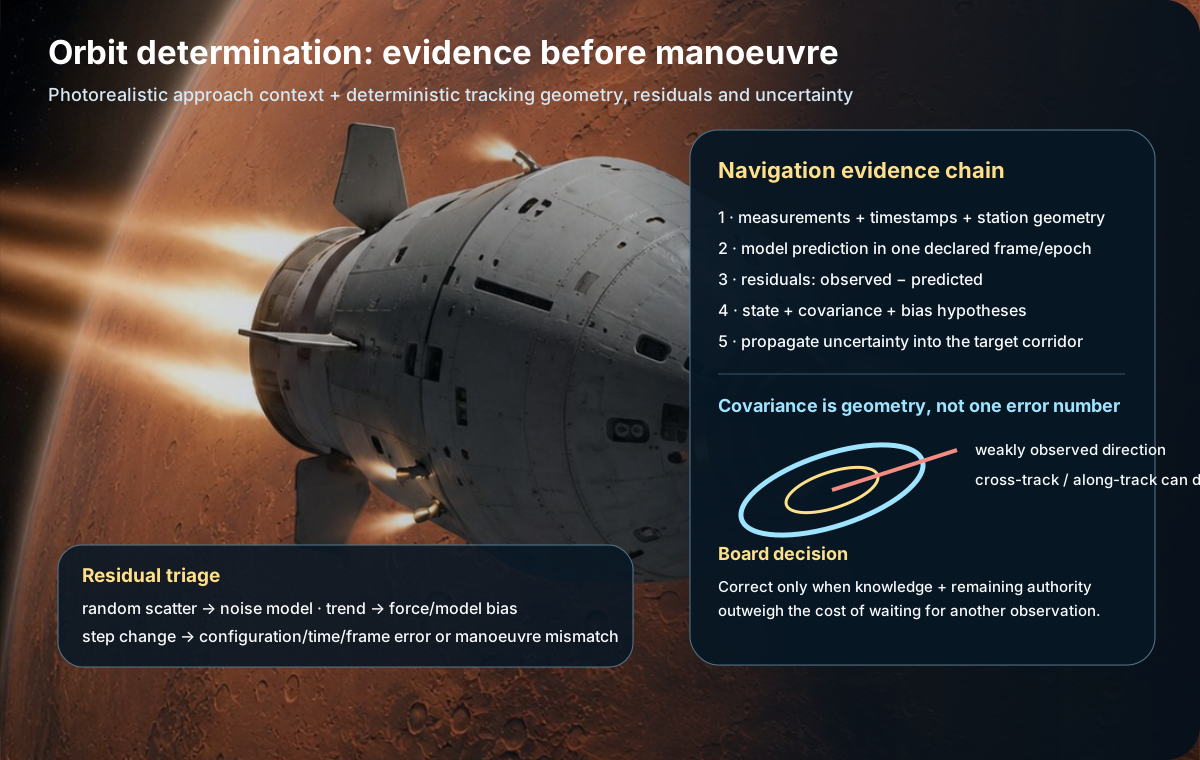
1. Tracking data are observations, not a trajectory
A range measurement, a Doppler measurement, an optical line of sight and a star-tracker attitude sample do not directly “give the orbit”. Each observation is produced at a time, from a sensor with calibration history, through a geometry that makes some directions easier to observe than others. Orbit determination begins by keeping that metadata attached to the number. If a tracking point loses its time tag or station geometry, it may become less useful than a noisier observation whose context is complete.
The practical lesson is to separate three layers. The first is the raw observation and its uncertainty. The second is the measurement model that predicts what the sensor should have observed for a candidate state. The third is the estimation process that changes the candidate state until the residual pattern becomes statistically and physically credible. A review board therefore asks not only “what is the state?” but “which measurements constrain each part of the state, what assumptions connect them to the model, and what unexplained structure remains in the residuals?”
JPL's Horizons documentation is useful here because it forces the reader to think in explicit epochs, coordinate systems and observer/target definitions rather than treating an ephemeris as a picture.
2. Covariance has shape because knowledge has direction
A single ± number is often a poor description of navigation knowledge. Tracking geometry may constrain radial position strongly while leaving along-track position weaker, or constrain plane orientation differently from range. The uncertainty therefore has structure. The covariance matrix is the bookkeeping object professionals use to retain that structure, but a beginner can first understand it as an uncertainty ellipsoid whose long axis points toward what the observations know least well.
The operational consequence is important. A state estimate can have a small overall summary metric and still be weak in the direction that matters for an upcoming targeting constraint. Conversely, one large uncertainty component may be harmless if it lies nearly tangent to a wide corridor. A command decision should therefore propagate uncertainty into the future constraint rather than declaring “navigation is good” from one scalar.
Correlations matter too. If two state components move together in the estimator, changing one without respecting the other can create impossible combinations. Monte Carlo sampling that ignores correlations can then exaggerate or hide risk. A competent review asks where the covariance came from, whether process noise and measurement noise are justified, and whether the uncertainty has been validated against residual behaviour.
3. Residuals are a diagnostic language
A residual is the difference between what a sensor observed and what the model predicted for the estimated state. Random scatter around zero may be consistent with the stated noise model. A trend can indicate an unmodelled force, a clock or calibration bias, a manoeuvre mismatch, or a poor state. A step change can point to a configuration event. Periodic structure may reveal geometry, thermal cycles or sensor behaviour. The residual plot is therefore not a decorative confirmation that the estimator ran; it is evidence about whether the model and data are telling the same story.
A disciplined triage first asks whether the anomaly is common to several sensors. If only one sensor family shifts, suspect that chain before changing the trajectory. If multiple independent sensors show compatible structure, the state or force model deserves more attention. If the anomaly appears immediately after a burn, reconstruct the burn before inventing a new environmental effect. This sequence protects the team from “fixing” the orbit to absorb a measurement problem.
4. A manoeuvre is not complete when the engine shuts down
The commanded burn contains a planned start time, direction, magnitude and duration or impulse target. The executed burn contains what the vehicle actually did. Those are not the same object. Finite thrust, attitude error, timing error, engine performance, valve transients and guidance cut-off logic can change the delivered velocity increment. Flight dynamics therefore needs a post-burn reconstruction using propulsion telemetry, attitude history and subsequent tracking.
The board then compares reconstructed performance with the navigation solution. If the propulsion reconstruction says the burn was nominal but tracking shows a miss, the discrepancy must be understood. If both agree on underperformance, the correction ledger is updated and the propulsion system may need follow-up. This avoids an easy but dangerous habit: treating every trajectory discrepancy as “navigation error”.
5. Correction timing trades knowledge against control authority
An early correction usually leaves more geometric and propellant authority but is made with less accumulated navigation information. A later correction can benefit from better measurements but may require a larger or more sensitive manoeuvre, leave less time for a recovery burn, or occur after a decision point that closes an option. The correct timing is therefore a trade, not a slogan such as “correct as soon as possible” or “wait for better data”.
The review should state what new information is expected before the next opportunity, how much the uncertainty is likely to shrink, how the manoeuvre cost and sensitivity change with time, and which contingency options disappear if the team waits. A protected correction budget should distinguish nominal correction, navigation dispersion, execution dispersion and contingency reserve so that waiting does not quietly spend the last recoverable option.
6. Target a corridor because every real requirement has width
A mission rarely needs one mathematically perfect point. Arrival states, interface conditions, lighting, communications, thermal limits, engine capability and downstream guidance create a feasible region. The centre of that region may be convenient for planning, but the review decision concerns whether the propagated state and uncertainty remain inside the protected envelope with sufficient margin.
This makes uncertainty directly operational. If the mean state is inside the corridor but a meaningful part of the uncertainty extends across a hard boundary, the team has not yet demonstrated compliance. It can improve knowledge, move the target deeper inside the envelope, change the corridor if the requirement allows it, or preserve more correction authority. A plot that shows only the nominal line hides the decision.
7. Time systems and frames are configuration-controlled mission data
Trajectory work is full of labels that look familiar but are not interchangeable: inertial frames, body-fixed frames, local orbital frames, barycentric descriptions, Earth time standards and spacecraft event time. A state vector is incomplete unless its frame and epoch are known. A manoeuvre vector is incomplete unless the direction convention is known. A navigation residual is ambiguous if its time standard is unclear.
Configuration control therefore belongs inside flight dynamics. A review package records the force model, gravity field version, ephemeris version, leap-second or time conversion data, software build and coordinate conventions. This is not paperwork added after the engineering. It is what allows another team to reproduce the state instead of trusting a screenshot produced by an unknown configuration.
8. Observability improves when measurements look from different directions
Adding more of the same measurement can reduce random noise without solving weak geometry. If the line of sight changes little, some combinations of position and velocity can remain hard to separate. A new tracking station, a later observation after geometry evolves, or an optical measurement with a different sensitivity can be more valuable than many repetitions of the same observable.
This is why a mission planner asks what information a measurement contributes, not only how precise the instrument is in isolation. The goal is to shrink the uncertainty that threatens the next decision. If along-track knowledge controls arrival timing, choose observations that improve along-track observability. If cross-track uncertainty threatens a corridor boundary, design the measurement campaign accordingly.
9. Model fidelity should be earned by the decision
A simple two-body model is ideal for intuition, unit checks and independent estimates. A high-fidelity propagator can include nonspherical gravity, third bodies, solar radiation pressure, atmospheric drag when relevant, relativity, finite manoeuvres and detailed ephemerides. More terms do not automatically make a better decision. The model should include effects that can materially move the answer relative to the margin being protected.
A useful discipline is to start with the simplest model that can expose the dominant mechanism, then add effects one by one and record how the decision variable changes. If a sophisticated term moves the target by a negligible amount compared with measurement uncertainty, it may not deserve operational attention yet. If a neglected term consumes a large part of the margin, the simple model has reached its boundary.
10. Monte Carlo is an uncertainty experiment, not a cloud of pretty trajectories
Monte Carlo analysis samples uncertain inputs and propagates many cases. Its value comes from the questions asked before the runs: which uncertainties are aleatory and which reflect lack of knowledge, which variables are correlated, what distribution is justified, what constitutes failure and how many samples are needed to characterise the tail relevant to the decision.
The board should identify the dominant contributors to failure cases rather than merely quote a percentile. If one calibration bias dominates the tail, an additional calibration may reduce risk more efficiently than a larger propellant reserve. If a hard constraint is violated by a tiny number of runs because the input model has an unrealistic distribution, the remedy is to correct the model, not hide the outliers.
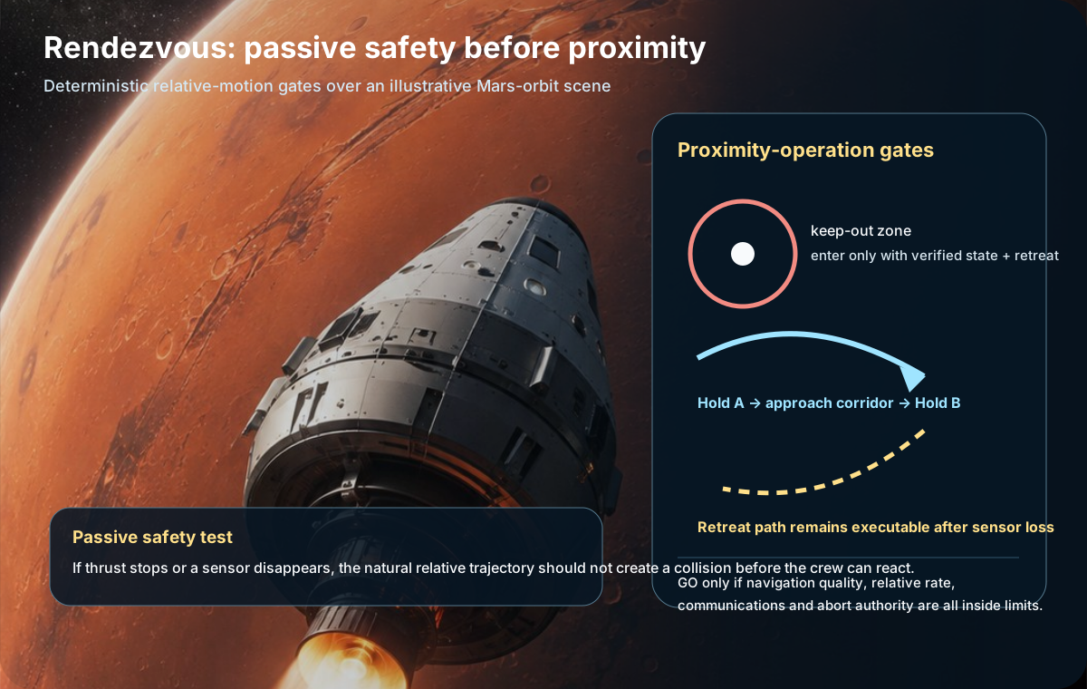
11. Rendezvous is a sequence of protected states
Rendezvous changes the safety logic because the target vehicle becomes a collision hazard. Passive safety means that loss of thrust or one expected control action should not immediately create a collision. Hold points create places where the team can stop, verify relative navigation, communications, attitude, propulsion and abort capability, then authorize the next approach segment.
The keep-out zone is not just a circle on a diagram. It represents a change in operational authority and failure tolerance. Inside it, smaller navigation errors and shorter response times matter. The crew or autonomous system must know the retreat manoeuvre, sensor fallbacks and conditions that trigger a stop. A good rendezvous plan therefore includes approach geometry, relative rates, lighting and sensor geometry, communication constraints and the natural relative trajectory if the next burn never occurs.
12. Abort geometry must be analysed before it is needed
An abort is not “burn away”. The direction that creates separation now can create an unsafe encounter later if orbital dynamics curve the relative trajectory back toward the target. The safe retreat path is therefore designed, propagated and rehearsed in advance. Its propellant, sensor and communications requirements belong in the nominal mission plan.
The same logic applies to Mars capture and flyby contingencies. If a capture burn underperforms, the spacecraft may enter an unexpected orbit or remain on a hyperbolic path. The team needs pre-analysed families of outcomes, not an improvised answer after the event. Those families define what telemetry to prioritise, when a correction remains possible and which states are unrecoverable with the protected reserve.
13. Numerical tools must produce a reviewable evidence package
Professional software is essential, but the output that supports a decision must be inspectable. A review package should include initial conditions, model settings, manoeuvre definitions, constraints, convergence criteria, uncertainty assumptions, residual summaries, sensitivity results and a versioned output. Independent hand checks remain valuable because they can reveal unit, sign or scale errors before a high-fidelity tool produces a very precise wrong answer.
The learner should be able to explain what the software was asked to solve, which constraints were active, what the solution is sensitive to and how the result was validated. “The optimiser converged” is not a mission argument.
14. Navigation handover is an engineering deliverable
A shift handover should allow the incoming team to recreate the state of knowledge: current authoritative state and covariance, frame and epoch, measurement arc, excluded data and reason, residual behaviour, manoeuvre history, protected correction budget, next observation opportunities, next decision time, open anomalies and ownership. If the incoming team cannot reproduce the propagation, the handover is incomplete.
The human factor matters. Important uncertainty should not exist only in one specialist's memory. The handover should distinguish known facts, current estimates, assumptions under test and unresolved contradictions. That structure reduces the chance that confidence is accidentally upgraded when a sentence loses its caveat across shifts.
15. Qualification casebook — twelve flight-dynamics board situations
- Range improves while Doppler residuals trend. Keep the state under review; a single observable looking better does not clear a model inconsistency.
- Two tracking stations disagree after a timing-system update. Freeze trajectory changes until the time/configuration chain is reconciled.
- Covariance shrinks but the arrival corridor is still crossed in the weak direction. Target the decision-space uncertainty, not a scalar uncertainty score.
- Burn telemetry indicates nominal duration but the reconstructed direction is biased. Update the achieved vector and investigate attitude/execution before blaming navigation.
- A later correction costs less propellant in the nominal case but leaves no recovery slot. Protect the recovery option unless the mission board explicitly accepts its loss.
- Monte Carlo failures cluster around one optical bias. Test calibration or measurement strategy before buying the entire bias with reserve.
- A high-fidelity model shifts arrival by more than the remaining corridor margin. The simple benchmark remains useful, but the higher-fidelity effect is now decision-relevant.
- Rendezvous relative navigation degrades at a hold point. Stay at the hold point or retreat; do not continue because the target is visually close.
- Abort burn creates immediate separation but a later re-encounter. Reject the abort geometry and redesign the passive-safe branch.
- Independent teams reproduce different state vectors. Compare frame, epoch, ephemeris and force-model configuration before comparing numbers.
- Propellant ledger has one reserve number. Split planned manoeuvres, expected correction, execution dispersion and protected contingency reserve.
- The plot looks smooth but a residual step appears after a software update. Treat configuration as a candidate cause and preserve the pre-update solution for comparison.
Escape speed — identify the zero-energy boundary without confusing it with “no gravity”
- 1 — Concrete question
- What local speed corresponds to the boundary between a bound two-body trajectory and a just-unbound trajectory?
- 2 — Intuition without symbols
- To coast away without another burn, the vehicle needs enough kinetic energy that its speed can approach zero arbitrarily far from the central body.
- 3 — Quantities first
- v_esc is local escape speed; μ is the gravitational parameter of the chosen central body; r is distance from that body’s centre.
- 4 — Formula
- v_esc = √(2μ/r)
- 5 — Read aloud
- Escape speed equals the square root of two mu divided by r.
- 6 — Symbols and meaning
- v_esc is a speed; μ represents the strength of the central gravity field; r is the current centre-to-centre distance.
- 7 — Pronunciation
- v escape equals square root of two mu over are.
- 8 — Units
- With μ in km³/s² and r in km, the result is km/s.
- 9 — Convention
- The speed is local and central-body-specific. It does not mean gravity disappears, and it is not the launch delta-v from a planetary surface.
- 10 — Why this operation
- Setting specific orbital energy to zero gives v²/2 − μ/r = 0, which rearranges to the escape-speed relation.
- 11 — Assumptions
- Two-body model, no atmosphere, no further thrust, and one clearly stated central body and reference frame.
- 12 — Unit check
- 2μ/r has units km²/s²; taking the square root gives km/s.
- 13 — Numerical case
- At a location where circular speed is 3.40 km/s, local escape speed is √2 × 3.40 ≈ 4.81 km/s.
- 14 — Why the calculation works
- The zero-energy boundary is √2 times local circular speed because circular specific energy is negative while the escape boundary is exactly zero.
- 15 — Algebra check
- Substituting v_esc² = 2μ/r into v²/2 − μ/r gives zero exactly.
- 16 — Mental estimate
- √2 is about 1.414, so a 3.4 km/s circular speed should imply an escape speed just under 4.9 km/s.
- 17 — Interpretation
- The value separates bound elliptical states from the parabolic boundary and positive-energy hyperbolic states in the ideal two-body model.
- 18 — What the result does not prove
- It does not provide launch losses, atmospheric drag, gravity losses, propulsion efficiency, ascent steering, or solar-system escape conditions.
- 19 — Sensitivity
- Escape speed falls with the inverse square root of radius; moving farther from the central body lowers the local boundary.
- 20 — Guided and autonomous practice
Guided exercise. Local circular speed is 3.40 km/s. Estimate escape speed from the same radius.
Guided correction
Use v_esc = √2 v_c. Thus 1.414 × 3.40 ≈ 4.81 km/s.
Autonomous exercise. Explain why a spacecraft can exceed Mars escape speed locally and still remain gravitationally bound to the Sun.
Autonomous correction
Orbital energy is defined relative to a chosen central body. A Mars-relative hyperbola may still have negative heliocentric energy and therefore remain on a bound solar orbit.
- 21 — Mission decision
- Always name the central body when using the phrase “escape speed”; do not turn a local energy boundary into an unqualified mission delta-v.
Primary sources: JPL Horizons documentation, JPL Solar System Dynamics orbit documentation, NASA Basics of Space Flight, and the NASA NTRS astrodynamics modelling reference.
Flight-dynamics qualification extension — the cases that separate a calculator from a navigator
Knowing the standard orbit equations is not enough to command a real trajectory. A navigator must know what was measured, what was assumed, how uncertain the state remains, which manoeuvre is still recoverable, and what evidence would cause the team to change its mind. The following qualification layer deliberately focuses on those judgement skills. It uses the equations already developed in their full mini-lessons rather than introducing unexplained symbolic shortcuts.
16. B-plane intuition for planetary arrival
A planetary arrival is easier to reason about when the team describes the incoming trajectory relative to the target planet rather than only as a heliocentric curve. Mission designers often use a target plane perpendicular to the asymptotic incoming velocity. A point on that plane summarizes where the unpowered incoming path would pass relative to the planet. The beginner does not need to memorize a specialist coordinate system on first contact; the important idea is that arrival targeting is two-dimensional and has direction. A miss can be too high, too low, or displaced sideways, and those directions can have very different consequences for atmosphere entry, orbital capture or flyby geometry.
For review-board work, the targeting picture should always expose at least four things: the chosen arrival aim point, the uncertainty region around it, the protected keep-out regions, and the manoeuvre authority still available to move the uncertainty region. A single nominal dot is not a plan. If the uncertainty ellipse overlaps a forbidden region, the board must either improve knowledge, move the target, preserve more correction authority or accept a different arrival mode.
17. Deterministic margins and statistical confidence answer different questions
A deterministic margin asks how far the nominal prediction remains from a hard limit after known allowances are applied. A statistical confidence region asks how uncertain the prediction is under a declared noise and error model. The two should not be merged into one comforting number. A large nominal margin can still be unsafe if the uncertainty is wider than the remaining clearance. Conversely, a broad uncertainty estimate does not automatically require a manoeuvre if additional tracking will shrink it before the last economical correction opportunity.
At a review, the analyst should state which uncertainty sources are represented, which are only bounded, and which are not modeled. Tracking noise, station geometry, clock error, manoeuvre execution error, force-model error and optical-centroid bias do not all behave alike. A credible board package names the dominant contributors instead of showing a colored ellipse with no provenance.
18. Finite burns are trajectories, not instantaneous punctuation marks
Introductory orbital mechanics often models a manoeuvre as an instantaneous velocity change. That approximation is useful because it isolates the geometry and energy logic. A real engine burns for a finite time while the vehicle continues moving under gravity. Thrust magnitude, direction, start time, cutoff time, mass flow and attitude history all matter. When the burn duration becomes non-negligible compared with the local orbital timescale, the impulsive approximation can no longer carry the entire targeting argument.
The operational discipline is therefore staged. Use the simple model to understand the manoeuvre and to make rapid sanity checks. Use the higher-fidelity propagation to design and predict the actual burn. After execution, reconstruct what the spacecraft really did from telemetry and tracking. The command package should preserve all three layers so that an unexpected result can be traced to physics, execution, navigation or configuration rather than hidden inside one software output.
19. Thrust uncertainty has direction as well as magnitude
An engine can underperform in total impulse, point slightly away from the commanded direction, start late, stop late, or combine several small errors. Those cases do not produce the same trajectory error. A shortfall parallel to the desired velocity change mostly alters the intended energy change; a transverse component can introduce plane or targeting error; timing error changes where along the orbit the thrust was applied. The navigator should therefore review the reconstructed vector and timing, not only the total delivered impulse.
Before a critical burn, define the telemetry and tracking evidence that will be available afterward. If the navigation team cannot distinguish magnitude error from pointing or timing error, the recovery strategy should reflect that ambiguity. A robust architecture preserves enough time and fuel to diagnose before committing to the next irreversible event.
20. Correction authority is a resource that expires
A correction that is cheap early can become expensive late because geometry evolves and because some future event has a fixed time. Waiting for better knowledge is valuable, but waiting too long can consume the remaining leverage. This creates a decision curve rather than a universal rule. Early in the approach, the team may prefer more observations. Near a final targeting gate, the same uncertainty may require action because the next opportunity is too weak or too late.
A board should therefore display correction authority as a function of time, not merely as “fuel remaining”. Include the remaining usable manoeuvre opportunities, the maximum correction each can safely deliver, navigation update latency, command validation time, communications constraints and protected reserves. The result turns a vague debate about waiting into an auditable timing decision.
21. Rendezvous relative navigation must degrade gracefully
Proximity operations depend on relative state knowledge. Different sensors dominate at different ranges: long-range tracking, optical line-of-sight information, range and range-rate sensors, lidar or radar where equipped, and finally close-range visual or fiducial cues. A robust plan does not assume one sensor works perfectly from acquisition to docking. It specifies the range and geometry in which each source is trusted, cross-checks between independent sources, and a retreat condition if the navigation solution becomes inconsistent.
Passive safety means the predicted free motion after a single failure should not immediately cause collision. That property must be examined at every hold point, not added as a sentence after the trajectory is designed. The safe branch includes time to detect the fault, time to decide, actuator authority to retreat, keep-out geometry, communications delays and the possibility that the target itself is off-nominal.
22. Communications latency changes who is allowed to decide
Deep-space operations cannot assume that Earth can intervene inside every hazard clock. The navigation organization therefore needs delegated authority and pre-agreed decision boundaries. The vehicle or local crew may be authorized to hold, abort, safe or execute a prevalidated contingency when the time available is shorter than a round-trip consultation. This is not “full autonomy” in the science-fiction sense; it is a carefully bounded allocation of authority based on time-criticality.
The flight-dynamics package should identify which decisions require ground concurrence, which can be executed locally, and which automatically trigger a safe state. Those rules belong beside the trajectory because the physical timeline determines whether a human organization can actually respond.
23. Configuration control is part of navigation truth
A trajectory solution is reproducible only when its configuration is known. Ephemeris version, force model, frame definition, epoch, spacecraft mass properties, manoeuvre file, sensor calibration, clock correction, software build and numerical tolerances can all change an answer. A review should be able to recreate the result later from a frozen evidence package. “The software gave this trajectory yesterday” is not sufficient evidence.
For high-consequence events, preserve an input manifest, configuration hashes or equivalent identifiers, the output products used for the decision, and a human-readable note explaining what changed since the previous solution. This practice also protects the team from silently comparing predictions produced with different assumptions.
24. A navigation anomaly is a hypothesis competition
When tracking disagrees with prediction, do not immediately tune the trajectory to fit the data. Competing hypotheses may include a real unmodeled force, a clock or station problem, a sensor bias, an incorrect manoeuvre reconstruction, a frame mismatch, data association error or a software/configuration defect. Each hypothesis predicts a different pattern across measurements and time.
The team should ask what independent observation could discriminate between them. A different station geometry, an optical measurement, telemetry from the propulsion system, a clock cross-check or a reprocessing run with frozen configuration may collapse the ambiguity. The best next action is often the observation with the highest diagnostic value, not the manoeuvre with the largest immediate effect.
25. Qualification board — twelve advanced flight-dynamics cases
- The residuals shrink but remain biased in one direction. Decide whether the force model, station geometry or measurement bias is the more credible explanation and specify the next discriminating observation.
- A late tracking pass halves the covariance but leaves only one economical correction window. Decide whether the knowledge gain compensates for the loss of future authority.
- Burn telemetry reports nominal duration but tracking reconstructs a cross-track error. Separate pointing, timing and navigation hypotheses before commanding another burn.
- Two orbit solutions agree on position but disagree on velocity. Explain why this can still produce rapidly diverging future predictions and identify the observation geometry needed next.
- A Mars arrival target is nominally centered but its uncertainty overlaps a protected atmospheric boundary. Re-target, improve knowledge or change arrival mode; do not declare GO from the nominal alone.
- An optical solution and radiometric solution disagree. Review calibration, geometry, timing and data association before averaging them together.
- One rendezvous sensor drops out inside a hold point. Determine whether the independent remaining sources support continuation or require retreat.
- The target vehicle cannot maintain the assumed attitude. Recompute passive-safety geometry and docking sensor visibility before continuing approach.
- Earth concurrence cannot arrive before the abort deadline. Apply the predelegated local authority and document which threshold triggered it.
- A high-fidelity propagator differs from the hand-check model. Identify which perturbation or finite-burn effect explains the difference instead of discarding the simple model as “wrong”.
- A software update changes the predicted correction by a small but operationally important amount. Freeze both configurations and reproduce the delta before accepting the new command.
- Fuel remains plentiful but only one geometry-correct correction opportunity remains. Treat time and geometry as the limiting resources, not tank quantity.
26. Final qualification exercise — from tracking arc to GO/HOLD/ABORT
You receive a short approach campaign containing radiometric tracking, an optical update, propulsion telemetry from the previous correction and two candidate future correction windows. Build the review as if another navigator must reproduce it. State the frame and epoch, identify the measurements that actually constrain the state, explain the covariance shape, classify residual patterns, state competing anomaly hypotheses, preserve a correction-authority timeline, show the arrival corridor and protected boundaries, and define the evidence required for GO, HOLD or ABORT.
The board should reject any answer that merely produces a trajectory plot. The required deliverable is an auditable chain from observation to model, from model to uncertainty, from uncertainty to risk, and from risk to a reversible mission decision. A competent navigator is not the person who knows the most equations by memory; it is the person who can show why a command is justified and how the mission remains safe if one assumption is wrong.
Primary source: JPL Horizons documentation, JPL orbit/ephemeris documentation, and NASA Basics of Space Flight.
Deep-space flight-dynamics qualification — from launch opportunity to Mars aim point
Module 05 already teaches the core equations of bound orbits, escape energy, plane change and hyperbolic arrival. This section connects those equations to the way a navigation team turns them into an interplanetary command product. Trajectory design, orbit determination, manoeuvre planning and arrival targeting are different activities that exchange evidence. A mission can have a mathematically elegant nominal trajectory and still be unsafe if its state estimate, uncertainty, correction authority or arrival corridor is not closed.
Design
Choose candidate departure and arrival epochs, solve boundary-value transfers, estimate launch energy, cruise duration and arrival state, then trade those against vehicle and operations constraints.
Navigation
Estimate the spacecraft state from tracking observations. Carry the epoch, reference frame and uncertainty with the state so that the trajectory line is never mistaken for perfect knowledge.
Control
Reserve trajectory-correction authority and schedule opportunities while the team still has both useful tracking information and enough time to recover from execution error.
Targeting
Translate the incoming asymptote into an aim point and corridor that the selected entry or capture architecture can actually tolerate.
1. A launch window is a constrained set of solutions, not a date printed on a calendar
The synodic rhythm explains why broad opportunities recur, but a usable launch window is created only after the mission computes actual trajectories across many departure and arrival epochs. A practical map often exposes the trade between launch energy, time of flight and arrival speed. The “best” cell depends on the mission: a cargo precursor can tolerate a different flight time from a crewed transfer; a launcher can be limited by characteristic energy; an arrival architecture can be limited by entry speed, capture propellant or lighting. The window is therefore a design surface with constraints, not a single celestial appointment.
A disciplined review preserves the ephemeris version, reference frame, departure and arrival states, force model and solver assumptions that generated the trade. If the launch-energy contour changes after an ephemeris or constraint update, the project should be able to reproduce why. This is the difference between a result and an auditable result.
2. Lambert or equivalent boundary-value targeting connects two planetary states over a chosen flight time
The Hohmann transfer remains valuable because it gives intuition and a benchmark. Real interplanetary targeting is more general: the planets are not ideal coplanar circles, launch and arrival dates are mission variables, and the spacecraft must connect two position states in a specified time. A Lambert solution or another boundary-value method supplies a transfer velocity consistent with those boundary conditions. Changing the time of flight changes the solution even if the endpoints remain similar.
This is why a trajectory team does not speak of “the” Earth–Mars transfer orbit as if one immutable ellipse existed. It speaks of a family of candidate trajectories, each with a departure state, arrival state, time of flight and associated constraints. The engineering review then asks which family member leaves enough margin for the launcher, propulsion, communications, thermal control, crew operations and arrival system.
3. Patched-conic reasoning is a sizing model whose boundaries must stay visible
Early design often separates the problem into a departure hyperbola around Earth, a heliocentric cruise, and an arrival hyperbola around Mars. This is useful because it connects launcher characteristic energy, interplanetary excess velocity and local arrival speed with simple physics. It becomes dangerous when those boundaries disappear from the documentation. A patched-conic number should be labelled as a sizing result, not silently promoted into a final command product.
Higher-fidelity propagation can include third-body gravity, oblateness where relevant, solar radiation pressure, manoeuvre duration and the exact mission ephemerides. The required fidelity depends on the decision. A preliminary launcher trade does not need the same model as the final pre-entry navigation solution. The qualification skill is choosing a model that is simple enough to understand and rich enough to support the decision.
4. Orbit determination is an evidence problem before it is a trajectory problem
A navigation state is an estimate built from observations. Range and Doppler tracking constrain different combinations of position and velocity; optical navigation or other data can add geometry. The estimate is tied to a specific epoch and reference frame. Its covariance or equivalent uncertainty description records what remains unresolved. A nominal trajectory without uncertainty cannot answer the operational question “how likely is the spacecraft to violate the corridor?”
Residuals matter because they test whether the measurements and the navigation model agree within expectations. A sudden residual pattern may indicate a bad observation, an unmodelled force, a manoeuvre execution error or a hardware problem. The response is not to “force the trajectory back onto the line.” The team first diagnoses whether the new estimate is credible, then propagates both the state and its uncertainty into the next decision.
5. Trajectory correction manoeuvres form a campaign, not a single midcourse event
NASA Mars missions routinely plan multiple opportunities to refine the cruise trajectory. The logic is general: launch injection is never exact, navigation knowledge improves with tracking, and the arrival target can become more demanding as the spacecraft approaches Mars. Early corrections remove large known errors efficiently; later opportunities trim the remaining miss after better observations arrive. Contingency slots protect the mission against a burn that underperforms or a state estimate that shifts.
The correction campaign should preserve a budget for both expected statistical clean-up and off-nominal recovery. A burn plan therefore carries the commanded vector, execution model, attitude constraints, propulsion mode, expected state change, protected reserve and post-burn tracking plan. The manoeuvre is not closed when the thrusters stop; it is closed when tracking reconstructs the delivered change and the updated state still supports the next gate.
6. Arrival targeting turns the incoming asymptote into a corridor decision
For planetary arrival, the navigation team needs a representation that makes miss geometry visible. The B-plane is a plane perpendicular to the incoming asymptotic velocity and is widely used for targeting planetary encounters. In practical terms, it lets the team describe where the incoming path is aimed relative to the planet before strong local curvature dominates. Entry missions then map that aim geometry into atmospheric-entry conditions; orbiters map it into periapsis, capture-burn and atmosphere-clearance constraints.
Uncertainty belongs on the same plot. A nominal aim point can be inside the target while part of the uncertainty region crosses a protected boundary. The decision then depends on probability, consequence, available correction authority and the reliability of the navigation update. This is why a late correction can be justified even when the nominal miss appears small.
7. Finite burns and execution errors separate the command from the delivered manoeuvre
Most textbook equations treat a manoeuvre as instantaneous. A real engine produces thrust for a finite duration while gravity continues to act and attitude control must keep the thrust direction within limits. Long burns may need to be modelled explicitly rather than represented as one impulse. Even short burns carry magnitude, direction and timing errors. Those dispersions belong in the post-burn prediction and in the amount of correction authority protected for later.
The flight-dynamics package should therefore distinguish commanded delta-v, predicted delivered delta-v and reconstructed delivered delta-v. If the difference is larger than expected, the team asks whether the cause is propulsion performance, attitude execution, timing, navigation estimation or modelling. Treating every miss as “just another orbital correction” can hide a developing subsystem fault.
8. End-to-end worked mission review — one nominal path, several gates
- Opportunity screen. Broad Earth–Mars recurrence says when to look. Ephemerides and transfer solutions then produce candidate departure/arrival pairs with characteristic energy, flight time and arrival excess speed.
- Launcher interface. Suppose the selected teaching case has C3 = 12 km²/s². The corresponding departure excess speed is about 3.46 km/s. That is an interface requirement, not the whole heliocentric solution.
- Cruise reserve. Protect a teaching correction reserve of 40 m/s rather than allocating every metre per second to the nominal plan. The exact real value is mission-specific; the pedagogical point is that statistical and contingency authority are tracked separately.
- Navigation update. A late tracking pass moves the estimated Mars aim point. The board examines residuals and uncertainty before deciding whether the shift is physical and whether a correction improves the protected corridor.
- Arrival state. For a teaching arrival with Mars-relative excess speed 2.6 km/s, local speed at a Mars-centred radius of 3,800 km is about 5.41 km/s using the hyperbolic-arrival relation already taught. That speed is an input to the arrival architecture, not a landing prediction.
- Post-burn verification. After each correction, reconstruct delivered delta-v and propagate the new state and uncertainty to the next gate. No burn is closed by command acknowledgement alone.
9. Flight-dynamics review table — what must be reproducible
| Artifact | Minimum content | Why the board needs it |
|---|---|---|
| State vector | Epoch, frame, position, velocity, units | Prevents a trajectory from becoming an untraceable screenshot. |
| Uncertainty | Covariance or equivalent dispersion definition and confidence convention | Shows whether the protected corridor is robust to what is not known. |
| Propagation model | Gravity bodies, perturbations, integration settings, ephemeris version | Makes the predicted state reproducible. |
| Manoeuvre definition | Epoch, vector/frame, finite/impulsive model, propulsion assumptions | Separates what was commanded from what was physically expected. |
| Execution reconstruction | Telemetry/tracking basis and delivered delta-v estimate | Closes the feedback loop after a burn. |
| Arrival target | B-plane or equivalent aim definition, corridor limits and uncertainty | Connects cruise navigation to entry or capture. |
| Reserve ledger | Nominal correction, statistical reserve, contingency reserve | Stops small routine corrections from silently consuming recovery capability. |
| Decision log | Approved option, rejected alternatives, assumptions, open actions | Allows the next shift to understand why the trajectory was accepted. |
Ellipse geometry from periapsis and apoapsis
- 1 — Concrete question
Given the closest and farthest Mars-centred radii of an orbit, how do you recover its semi-major axis and eccentricity before calculating timing or manoeuvre consequences?
- 2 — Intuition without symbols
An ellipse can be described by how close it comes to the planet and how far it recedes. The midpoint of those two distances sets the overall size of the ellipse, while their contrast tells how stretched the orbit is.
- 3 — Quantities first
r_p is periapsis radius from the centre of the body; r_a is apoapsis radius; a is semi-major axis; e is dimensionless eccentricity.
- 4 — Formula
a = (r_p + r_a)/2 ; e = (r_a - r_p)/(r_a + r_p)- 5 — Read aloud
“a equals periapsis radius plus apoapsis radius divided by two; eccentricity equals apoapsis radius minus periapsis radius divided by their sum.”
- 6 — Symbols
The subscripts p and a mean periapsis and apoapsis. Semi-major axis a has units of length. Eccentricity e is a ratio and therefore has no unit.
- 7 — Pronunciation
Say r sub p, r sub a, a, and e. State explicitly that every radius is measured from the same central body and not from the surface.
- 8 — Units
The semi-major-axis expression keeps kilometres if both radii are in kilometres. The eccentricity expression divides a length by a length and is dimensionless.
- 9 — Convention
Use centre-to-centre radius, not altitude. If the inputs are altitudes, add the same reference-body radius to both before using the equations.
- 10 — Why this operation
A bound Keplerian ellipse is symmetric about its major axis. Periapsis and apoapsis sit at opposite ends, so their average gives the semi-major axis; their normalized difference measures the elongation.
- 11 — Assumptions
This is an osculating two-body description at one epoch. It ignores perturbations, atmosphere, finite burns and uncertainty unless those are added separately.
- 12 — Unit check
The first result must be a length. The second must be dimensionless and, for a bound non-degenerate ellipse, lie between zero and one.
- 13 — Numerical case
r_p = 4,000 kmr_a = 8,000 kma = (4,000 + 8,000)/2 = 6,000 kme = (8,000 - 4,000)/(8,000 + 4,000) = 0.333- 14 — Why each operation
Add the apsis radii to locate their midpoint, then halve the sum. For eccentricity, compare the apsis separation with their total scale; that normalization prevents a large orbit from looking more eccentric merely because all distances are larger.
- 15 — Algebra check
Recover the apsides with r_p = a(1-e) and r_a = a(1+e). With a = 6,000 km and e = 1/3, the recovered values are 4,000 km and 8,000 km.
- 16 — Mental estimate
The midpoint of four and eight thousand is obviously six thousand. The orbit differs by four thousand across a twelve-thousand total scale, so an eccentricity near one third is plausible.
- 17 — Interpretation
The orbit is moderately eccentric rather than nearly circular. Its timing, speed and burn effectiveness will differ substantially between periapsis and apoapsis.
- 18 — What it does not prove
The pair does not reveal orbital plane, orientation in the plane, spacecraft position, direction of motion or navigation uncertainty. Two spacecraft can share the same a and e and still be nowhere near rendezvous.
- 19 — Sensitivity or limit case
If apoapsis rises while periapsis is held fixed, both semi-major axis and eccentricity increase. If the two radii converge, eccentricity approaches zero.
- 20 — Practice
Guided exercise. An orbit has r_p = 3,800 km and r_a = 5,800 km. Find a and e.
Guided correction — open after your attempt
- a = (3,800 + 5,800)/2 = 4,800 km.
- e = (5,800 - 3,800)/(5,800 + 3,800) = 2,000/9,600 ≈ 0.208.
- Check: 4,800(1-0.208) ≈ 3,802 km and 4,800(1+0.208) ≈ 5,798 km; rounding explains the few kilometres.
Autonomous exercise. Choose a Mars-centred periapsis radius safely above the surface and an apoapsis radius at least twice as large. Compute a and e, then explain whether a plane change would be cheaper near periapsis or apoapsis and why.
Autonomous correction — open after your attempt
- A valid answer must use centre radii and produce 0 ≤ e < 1.
- Use vis-viva qualitatively: speed is lower near apoapsis, so the same pure plane-angle change generally costs less delta-v there.
- State that the best mission design still depends on where the required geometry and later manoeuvres must occur.
- 21 — Mission decision
Do not approve an “elliptical orbit” description that gives only altitudes. Preserve centre radii, a, e, epoch and orientation so downstream timing and manoeuvre calculations are reproducible.
Synodic period — estimate how often planetary geometry repeats
- 1 — Concrete question
How can a first-pass mission planner estimate the recurrence time of similar Earth–Mars angular geometry before using full ephemerides for an actual launch window?
- 2 — Intuition without symbols
Two planets move around the Sun at different rates. One gradually gains angular position on the other until their relative arrangement repeats. The repetition time depends on the difference between their orbital rates, not on either year length by itself.
- 3 — Quantities first
P_1 and P_2 are the orbital periods of the two bodies in the same time unit; S is the synodic period, the interval between repeating relative configurations in the idealized periodic model.
- 4 — Formula
1/S = |1/P_1 - 1/P_2|- 5 — Read aloud
“one over S equals the absolute value of one over period one minus one over period two.”
- 6 — Symbols
P denotes orbital period and S denotes synodic period. The absolute value removes the sign because a recurrence interval is positive.
- 7 — Pronunciation
Say “one over S” and “absolute value”. Name the bodies when reading the equation in a review so that period one and period two cannot be swapped silently.
- 8 — Units
Each reciprocal period has units of inverse time. Their difference is inverse time; taking the reciprocal returns a time.
- 9 — Convention
Use the same time unit for both periods. Treat this as a recurrence estimate, not as a precise launch-window date.
- 10 — Why this operation
Relative angular rate is the difference between the two mean orbital rates. The time required for relative phase to advance by a complete cycle is the reciprocal of that rate difference.
- 11 — Assumptions
The estimate treats the orbital periods as stable and compresses real eccentric, inclined planetary motion into a simple periodic relation. Mission targeting still requires ephemerides and a trajectory solution.
- 12 — Unit check
If periods are supplied in days, S must emerge in days. If the two periods were identical, the denominator would approach zero and the recurrence time would grow without bound.
- 13 — Numerical case
P_Earth = 365.25 dP_Mars = 686.98 d1/S = |1/365.25 - 1/686.98|S ≈ 779.9 d ≈ 2.14 years- 14 — Why each operation
Convert both motions to reciprocal periods before subtracting because what matters is relative rate. Take the reciprocal only after finding the magnitude of that difference.
- 15 — Algebra check
Insert S ≈ 779.9 d into the left side: 1/S ≈ 0.001282 d⁻¹. The difference of the two reciprocal periods is approximately the same value.
- 16 — Mental estimate
Earth completes roughly two years while Mars completes a little more than one. A relative-geometry repetition a little above two Earth years is therefore reasonable.
- 17 — Interpretation
Similar broad Earth–Mars geometry recurs on a roughly 780-day rhythm, which explains why launch opportunities are clustered rather than available on demand.
- 18 — What it does not prove
The number does not identify the best departure day, time of flight, C3, arrival speed, declination, launch-site constraints or the width of a usable launch window. Those require ephemerides and trajectory optimization.
- 19 — Sensitivity or limit case
If the two orbital periods were closer to one another, their relative angular rate would be smaller and the synodic period longer.
- 20 — Practice
Guided exercise. Use P_1 = 365 d and P_2 = 730 d. Estimate S.
Guided correction — open after your attempt
- 1/S = |1/365 - 1/730| = |2/730 - 1/730| = 1/730 d⁻¹.
- Therefore S = 730 d.
- The exact arithmetic is easy here because the second period is twice the first.
Autonomous exercise. Choose two hypothetical planetary periods that differ by less than 20%. Compute the synodic period and explain why similar orbital periods can produce a very long recurrence interval.
Autonomous correction — open after your attempt
- Convert both periods to the same unit and subtract their reciprocals.
- A small reciprocal-rate difference produces a large value when inverted.
- State clearly that the result predicts recurrence of relative phase in the simplified model, not a complete mission launch solution.
- 21 — Mission decision
Use synodic period to plan when broad opportunities recur, but never publish a launch date from it alone. Move to ephemerides, Lambert or equivalent targeting, and launch/arrival constraint maps for mission decisions.
Vector impulse — combine speed change and direction change
- 1 — Concrete question
When a burn changes both the magnitude and direction of velocity, how do you estimate the required impulsive delta-v instead of adding two scalar speed changes?
- 2 — Intuition without symbols
Velocity points somewhere; it is not only a speed. If the spacecraft must leave one velocity arrow and end on another, the burn is the vector gap between those arrows. A small turn at high speed can therefore cost more than intuition based on speed difference alone suggests.
- 3 — Quantities first
v_1 is the pre-burn speed, v_2 the post-burn speed, θ the angle between the velocity directions, and Δv the magnitude of the instantaneous velocity change.
- 4 — Formula
Δv = √(v_1² + v_2² - 2 v_1 v_2 cos θ)- 5 — Read aloud
“delta-v equals the square root of v one squared plus v two squared minus two v one v two cosine theta.”
- 6 — Symbols
The angle θ is the included angle between the two velocity vectors. Delta-v is a vector change whose magnitude is shown by this law-of-cosines relation.
- 7 — Pronunciation
Say “delta vee”, “cosine theta”, and state the angular unit used by the calculator. Degrees entered into a radian-mode calculator will invalidate the result.
- 8 — Units
Every squared-speed term has units of speed squared; the square root returns a speed such as kilometres per second.
- 9 — Convention
The relation treats the manoeuvre as impulsive and compares velocity vectors at one point and epoch in one reference frame.
- 10 — Why this operation
The initial velocity, final velocity and required change form a triangle in velocity space. The law of cosines gives the length of the change vector.
- 11 — Assumptions
Finite burn duration, gravity losses, attitude-transient constraints, thrust limits and execution dispersion are not included. They belong in a later manoeuvre model.
- 12 — Unit check
The terms inside the square root must all have units of speed squared. The result cannot exceed v_1 + v_2 and cannot be smaller than the absolute scalar speed difference.
- 13 — Numerical case
v_1 = 3.5 km/sv_2 = 3.5 km/sθ = 10°Δv = √(3.5² + 3.5² - 2×3.5×3.5×cos 10°) ≈ 0.610 km/s- 14 — Why each operation
Square both speed magnitudes, subtract the dot-product term that accounts for their alignment, then take the square root to return from squared-speed space to a delta-v magnitude.
- 15 — Algebra check
For equal speeds, the expression can be transformed to Δv = 2v sin(θ/2). With v = 3.5 km/s and θ/2 = 5°, this gives about 0.610 km/s again.
- 16 — Mental estimate
A ten-degree turn is modest, so delta-v should be much smaller than 3.5 km/s but not zero. Roughly six-tenths of a kilometre per second is credible.
- 17 — Interpretation
Changing direction alone can consume a large manoeuvre budget when the spacecraft is moving quickly. This is why plane changes are often scheduled where orbital speed is lower.
- 18 — What it does not prove
The equation does not tell you where to perform the burn, whether the target orbit is reachable with one impulse, how long the burn lasts, or whether navigation and propulsion can deliver the commanded vector.
- 19 — Sensitivity or limit case
At fixed speed, delta-v grows with turn angle. At fixed angle, it grows roughly in proportion to speed, making high-speed geometry changes expensive.
- 20 — Practice
Guided exercise. At one point, speed remains 2.0 km/s but direction must rotate by 30°. Estimate the impulsive delta-v.
Guided correction — open after your attempt
- Use the equal-speed form Δv = 2v sin(θ/2).
- Δv = 4.0 × sin 15° ≈ 4.0 × 0.2588 ≈ 1.04 km/s.
- Check that 1.04 km/s is below 4.0 km/s and above zero.
Autonomous exercise. Compare a 15° direction change at 2 km/s with the same turn at 6 km/s. Compute both and use the result to recommend where in an eccentric orbit a pure plane change should be placed when geometry allows.
Autonomous correction — open after your attempt
- At 2 km/s: Δv = 4 sin 7.5° ≈ 0.522 km/s.
- At 6 km/s: Δv = 12 sin 7.5° ≈ 1.566 km/s.
- The high-speed case costs three times as much because the speeds differ by a factor of three; prefer the slower orbital location if the mission geometry permits.
- 21 — Mission decision
Treat manoeuvres as vector changes. Before approving a burn, preserve the pre- and post-burn velocity vectors, frame, epoch, finite-burn assumptions and execution-error reserve rather than quoting a scalar delta-v alone.
Synthesis — relative orbital dynamics and propagation
These three mini-lessons consolidate relations that were previously scattered through the course. Earlier occurrences now remain as explanations or applications and refer back to these lessons.
Specific angular momentum — cross-check orbital plane and transverse motion
- 1 — Concrete question
- How can position and velocity direction be combined into a quantity that is conserved in the ideal two-body model?
- 2 — Intuition without symbols
- An orbital state carries a geometric signature: distance from the central body and the sideways part of the velocity together define how the trajectory sweeps around the centre.
- 3 — Quantities first
- The position vector points from the central body to the spacecraft; the velocity vector gives instantaneous motion; specific angular momentum combines them.
- 4 — Formula
- ⃗h = ⃗r × ⃗v ; if ⃗r ⟂ ⃗v, then h = r v
- 5 — Read aloud
- Specific angular momentum is the cross product of position and velocity; in the simple perpendicular case its magnitude is radius times speed.
- 6 — Symbols and meaning
- ⃗h is specific angular momentum, ⃗r is position, and ⃗v is velocity. Its direction is normal to the orbital plane by the right-hand rule.
- 7 — Pronunciation
- h vector equals r vector cross v vector.
- 8 — Units
- With r in kilometres and v in kilometres per second, h is in square kilometres per second.
- 9 — Convention
- The cross product depends on the angle between position and velocity; the shortcut h = r v is valid only when they are perpendicular.
- 10 — Why this operation
- The cross product isolates the velocity component that sweeps around the centre rather than pure radial motion.
- 11 — Assumptions
- Instantaneous state in a defined inertial frame; exact conservation additionally assumes central force only and no thrust.
- 12 — Unit check
- km multiplied by km/s gives km²/s; spacecraft mass does not appear because the quantity is specific.
- 13 — Numerical case
- At r = 4,000 km with a purely tangential speed of 3.30 km/s, h = 13,200 km²/s.
- 14 — Why the calculation works
- All of the velocity contributes because it is perpendicular to the radius; 4,000 × 3.30 gives 13,200.
- 15 — Algebra check
- In the tangential case v = h/r. A plane change rotates the direction of ⃗h even when its magnitude changes little.
- 16 — Mental estimate
- 4,000 × 3.3 is about 13,000, so a result of order 10⁴ km²/s is expected.
- 17 — Interpretation
- The magnitude tracks transverse orbital motion while the vector direction identifies the ideal orbital plane.
- 18 — What the result does not prove
- h alone does not determine orbital energy, exact location on the orbit, perturbations, or measurement error.
- 19 — Sensitivity
- A small error in tangential velocity maps directly into h; a direction error can rotate the vector without strongly changing its magnitude.
- 20 — Guided and autonomous practice
Guided exercise. At 5,000 km radius a spacecraft has 2.8 km/s purely tangential velocity. Compute h.
Guided correction
h = 5,000 × 2.8 = 14,000 km²/s.
Autonomous exercise. Two states have the same radius and speed, but one has a large radial component. Can h = r v be used for both?
Autonomous correction
No. Use the full cross product because only the velocity component perpendicular to the radius contributes to the magnitude of h.
- 21 — Mission decision
- Use angular momentum as an independent check of plane and transverse motion, never as a substitute for the complete state.
Relative motion and phase — determine whether two vehicles meet at the right place and time
- 1 — Concrete question
- How can separation from a target be quantified and a simple phase drift projected?
- 2 — Intuition without symbols
- Rendezvous requires more than similar orbits. The crew must know where the target is relative to the chaser, how that offset is changing, and whether relative rotation closes at the planned time.
- 3 — Quantities first
- Track relative position, relative velocity, an initial phase angle, and average angular rates over the simplified interval.
- 4 — Formula
- Δ⃗r = ⃗r_c − ⃗r_t ; Δ⃗v = ⃗v_c − ⃗v_t ; Δφ(t)=Δφ₀+(n_c−n_t)Δt
- 5 — Read aloud
- Relative state comes from subtracting target from chaser; simple phase drift evolves with angular-rate difference times elapsed time.
- 6 — Symbols and meaning
- Δ⃗r and Δ⃗v are position and velocity offsets; Δφ is phase angle; n_c and n_t are mean angular rates; Δt is elapsed time.
- 7 — Pronunciation
- delta r vector, delta v vector, then delta phi equals delta phi zero plus n chaser minus n target times delta t.
- 8 — Units
- Positions share one length unit, velocities one length-per-time unit, angles one convention, and angular rates angle per unit time.
- 9 — Convention
- All vectors must use the same frame and compatible epochs; the linear phase model is only a local approximation.
- 10 — Why this operation
- Subtraction removes the common absolute location and exposes separation; angular-rate difference gives how quickly phase closes or opens.
- 11 — Assumptions
- Orbits are regular enough for an average-rate model, no unmodelled burns occur, and vectors share frame and epoch.
- 12 — Unit check
- Position minus position remains position; velocity minus velocity remains velocity; angular rate times time gives an angle.
- 13 — Numerical case
- Two vehicles are 20° apart and the chaser gains 0.5° per equivalent interval. About 40 intervals are required to close 20° in this model.
- 14 — Why the calculation works
- Each interval removes 0.5°; 20 divided by 0.5 gives 40, with sign chosen consistently with the phase convention.
- 15 — Algebra check
- If the angular rates become equal, the drift term vanishes and phase remains constant in this simplified model.
- 16 — Mental estimate
- Closing roughly half a degree per interval across twenty degrees must take several tens of intervals, not two or three.
- 17 — Interpretation
- The calculation shows whether relative geometry evolves in the correct direction and gives a first-order time to alignment.
- 18 — What the result does not prove
- It does not replace linearised relative-motion dynamics, three-dimensional relative navigation, or approach-safety constraints.
- 19 — Sensitivity
- When angular-rate difference becomes very small, closure time becomes highly sensitive to period and measurement error.
- 20 — Guided and autonomous practice
Guided exercise. A 12° phase offset closes at 0.3° per hour. Estimate the time.
Guided correction
12/0.3 = 40 h in the average-rate model.
Autonomous exercise. Explain why two spacecraft at the same position but with different velocities are not yet in a safe rendezvous state.
Autonomous correction
Relative velocity is not zero, so separation immediately starts growing again and the encounter may be unsafe.
- 21 — Mission decision
- A rendezvous GO requires compatible relative position, relative velocity, and phase trend inside the approach corridor.
Numerical propagation — advance an orbital state without confusing a model with truth
- 1 — Concrete question
- How can a position-velocity state be advanced in time while checking that numerical integration remains credible?
- 2 — Intuition without symbols
- Propagation starts from the state known now, computes acceleration from the chosen model, and advances position and velocity step by step. A smooth plot is not proof: convergence and expected invariants must be checked.
- 3 — Quantities first
- Position vector, velocity vector, total acceleration, time, integration step, and selected perturbations form the calculation core.
- 4 — Formula
- d⃗r/dt = ⃗v ; d⃗v/dt = ⃗a_total ; ⃗a_total = ⃗a_2body + ⃗a_pert
- 5 — Read aloud
- The derivative of position is velocity; the derivative of velocity is total acceleration, here decomposed into central and retained perturbing terms.
- 6 — Symbols and meaning
- ⃗r and ⃗v form the dynamic state at an epoch; ⃗a_total is the acceleration used by the integrator; perturbation terms depend on model fidelity.
- 7 — Pronunciation
- d r vector over d t equals v vector; d v vector over d t equals total acceleration vector.
- 8 — Units
- Position is length, velocity length per time, acceleration length per time squared; the integration step uses a compatible time unit.
- 9 — Convention
- Frame, epoch, central body, constants, and force models are part of the computational state and must be version-controlled.
- 10 — Why this operation
- A differential equation gives a rate of change. The integrator reconstructs evolution by accumulating those changes with a chosen step and method.
- 11 — Assumptions
- Initial state is sufficiently known, force models match the time horizon, and step/tolerances match required accuracy.
- 12 — Unit check
- The derivative of length gives velocity and the derivative of velocity gives acceleration. Every acceleration term has the same dimension.
- 13 — Numerical case
- A bound two-body propagation is recomputed with time steps of
60 s,30 s, and15 s. The final position differs by42 mbetween 60 s and 30 s, then by only11 mbetween 30 s and 15 s. Against a mission tolerance of1,000 m, the 42 m difference is only4.2%of tolerance, and the next refinement reduces the discrepancy to11/42 ≈ 0.26of the previous value. The clear decrease in step-size sensitivity as the step is halved is the explicit numerical convergence test. - 14 — Why the calculation works
- If the solution converges as the step shrinks and ideal invariants remain stable in a test case, the integration is consistent with the required accuracy.
- 15 — Algebra check
- In a pure two-body coast, specific energy and angular momentum should remain nearly constant; drift indicates numerical or modelling error.
- 16 — Mental estimate
- Halving the time step should change the result by less than the navigation margin. A larger change means the coarser result is not robust.
- 17 — Interpretation
- Propagation turns a dated state into a predicted trajectory and supports event, window, correction, and margin analysis.
- 18 — What the result does not prove
- It does not prove that unmodelled forces are negligible, the initial state is correct, or the software is bug-free.
- 19 — Sensitivity
- Longer horizons allow small state, constant, and force-model errors to accumulate; update cadence must reflect this sensitivity.
- 20 — Guided and autonomous practice
Guided exercise. A trajectory changes by 4 km when the step is reduced from 60 s to 30 s, while targeting tolerance is 1 km. Is the 60 s step acceptable?
Guided correction
No. Step-size sensitivity exceeds the mission tolerance; continue the convergence study or change the integration method.
Autonomous exercise. In a two-body test, specific energy drifts steadily even with a small step. Name two causes to investigate.
Autonomous correction
Check integration method/step and unit or constant consistency first. A spurious force term or frame error could also cause the drift.
- 21 — Mission decision
- Qualify a propagated trajectory only after numerical convergence, expected invariant behaviour in test cases, and full force-model traceability.
Primary bridges for this extension
- NASA/JPL — B-plane targeting illustrated for Mars Science Laboratory
- NASA/JPL — interplanetary cruise and trajectory-correction manoeuvres
- NASA — Perseverance route to Mars and planned trajectory corrections
Validation rule for module 05. A learner is not qualified by reproducing a transfer equation alone. They must connect geometry, state estimation, uncertainty, manoeuvre authority and arrival targeting into an auditable navigation chain.