


Earth → Mars: windows, transfer, corrections and arrival
Connect launch energy to interplanetary geometry
Starting question — How do launch windows, phase angle, C3 and trajectory corrections determine whether an Earth–Mars transfer is feasible?
Intuition. Interplanetary flight is a timing problem as much as a propulsion problem: Earth, Mars and the spacecraft must arrive at compatible geometry while respecting launch-energy limits.
- Explain the governing physical idea before calculating.
- Name every symbol and unit used in the key relation.
- Check the result with an independent inverse, bound or order-of-magnitude test.
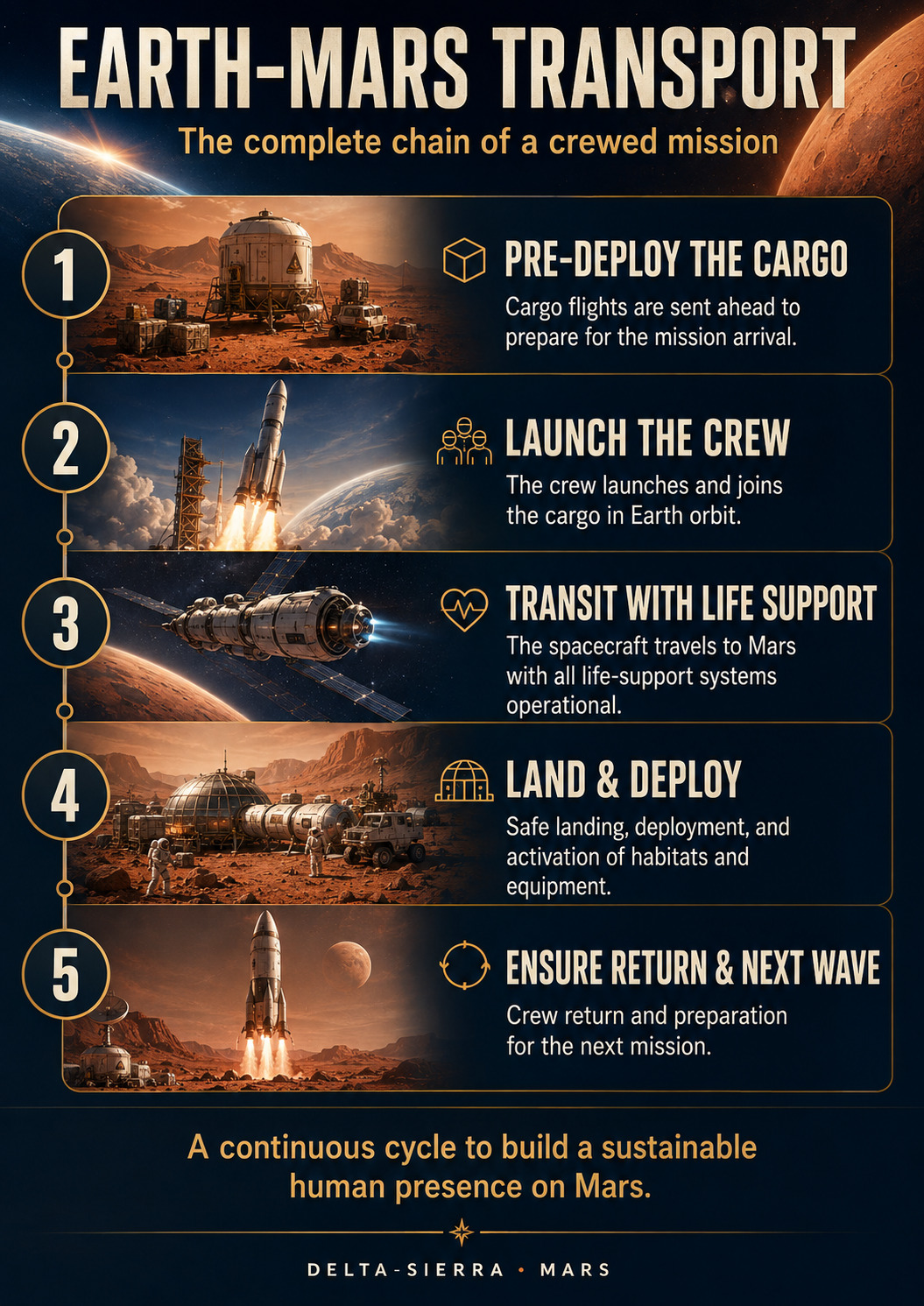
Travel from Earth to Mars is not “aim at Mars and fire the engines.” Both planets move around the Sun and the interplanetary path is itself a solar orbit. This module connects synodic period, launch window, Hohmann transfer, hyperbolic excess speed, trajectory correction and arrival.
1. Why windows repeat about every 26 months
Earth orbits in about 365.25 days and Mars in about 686.98 days. The synodic period S satisfies 1/S = |1/PE − 1/PM|.
Exercise A
Earth’s orbital period is 365.25 days and Mars’s is 686.98 days. Using S = 1 / |1/T_E − 1/T_M|, calculate the Earth–Mars synodic period in days and months. Then explain what this period does—and does not—tell you about a real launch window.
Detailed correction — Exercise A
Calculation. 1/365.25 ≈ 0.002738 day⁻¹ and 1/686.98 ≈ 0.001456 day⁻¹. Their difference is ≈0.001282 day⁻¹, so S ≈ 780 days ≈25.6 months.
Interpretation. The synodic period explains the approximate repetition of Earth–Mars geometry. A real launch window also depends on trajectory energy, vehicle capability, arrival constraints and planetary ephemerides.
Derive the synodic period instead of memorising it
If Earth and Mars orbit the Sun with periods Tₑ and Tₘ, their average angular rates are nₑ = 2π/Tₑ and nₘ = 2π/Tₘ. Their relative angular rate is |nₑ - nₘ|, so synodic period S satisfies 1/S = |1/Tₑ - 1/Tₘ|. With Tₑ ≈ 365.25 days and Tₘ ≈ 686.98 days, S is about 780 days, roughly 26 months. This explains why broadly similar geometries repeat without claiming that every window is identical. Orbital eccentricity and inclination, launch-vehicle capability, arrival constraints and mission objectives move the best departure date within each opportunity. The formula gives the cadence; trajectory design still has to solve the particular window.
2. Solar Hohmann transfer
In a circular coplanar model, the transfer ellipse has perihelion at 1 AU and aphelion near 1.524 AU. Its semimajor axis is about 1.262 AU and half its orbital period gives roughly 259 days, about 8.5 months. Real missions can trade flight time against launch and arrival energy.
3. Earth must lead the moving target
The spacecraft takes months to reach Mars’ orbit, so Mars must be ahead of the intersection point at departure by the correct phase angle. This is orbital mechanics’ version of aiming ahead of a moving target.
A heliocentric transfer has an energy condition at both ends
A simplified Earth–Mars transfer is an ellipse around the Sun. At departure the spacecraft must leave Earth with a heliocentric velocity different from Earth’s; at arrival it reaches Mars with a velocity different from Mars’s. The asymptotic planet-relative difference is v∞, measured in km/s. Launch characteristic energy C3 is v∞² and is measured in km²/s². C3 is therefore not a speed; it is a convenient measure of hyperbolic departure energy beyond a simple Earth orbit. Lower departure energy can imply a longer flight or a different arrival energy. Mission design has to evaluate both ends together because propulsion saved near Earth may reappear as capture, entry or thermal demand at Mars.
4. C3 and v∞
After escaping Earth’s immediate gravity well, the spacecraft has hyperbolic excess velocity v∞ relative to Earth. C3 = v∞². If v∞ is in km/s, C3 is in km²/s².
Exercise B
A departure trajectory has hyperbolic excess speed v∞ = 3.6 km/s relative to Earth. Calculate C3, keep the squared units explicit, and explain why this is not the complete ground-to-space velocity requirement.
Detailed correction — Exercise B
Calculation. C3 = v∞² = (3.6 km/s)² = 12.96 km²/s².
Interpretation. C3 describes hyperbolic excess energy relative to Earth. The launch system must still reach the required departure state while accounting for Earth gravity, atmosphere and steering losses.
C3 and v∞ connect launch vehicle and interplanetary trajectory
Hyperbolic excess speed v∞ is the spacecraft’s asymptotic speed relative to Earth after escaping the immediate gravity well. Characteristic energy C3 = v∞² is therefore measured in km²/s². If v∞ = 3.2 km/s, C3 = 10.24 km²/s². Launch-vehicle performance tables often use C3 because it captures how demanding the departure trajectory is beyond reaching low Earth orbit. Higher C3 usually means less payload for a given launcher. Mission design must then connect this departure condition to heliocentric trajectory and Mars arrival speed. A launch solution that looks attractive in Earth-centred coordinates can create an arrival condition that is expensive or thermally difficult at Mars.
5. Trajectory corrections manage injection error
Real injection is imperfect. Trajectory correction manoeuvres reduce the difference between estimated trajectory and target. Early corrections can be Δv-efficient but require enough tracking information to distinguish a real bias from measurement uncertainty.
6. Reaching Mars is not the same as being captured
An unbraked arrival is hyperbolic relative to Mars. Remaining requires propulsive capture, atmospheric energy dissipation, or another mechanism. A direct entry instead targets a narrow atmospheric corridor. Departure choice affects Mars v∞ and therefore arrival severity.
A small early correction can avoid a large late one
Injection never delivers exactly the planned state. A trajectory correction changes selected velocity components so that the evolving uncertainty remains inside the arrival target. Timing matters: months before Mars, centimetres per second can move the predicted encounter by thousands of kilometres, while the same correction hours before arrival has far less geometric leverage. Navigation should not chase every measurement fluctuation. The estimated state has a covariance, a mathematical description of uncertainty and correlation. A correction decision compares Δv cost with useful reduction of future target error, while preserving reserve for later manoeuvres. This is why navigation, guidance and propulsion planning cannot be separated into independent checklists.
7. A missed window can reshape the mission
For a crewed campaign, planetary geometry constrains production, testing, cargo, crew and reserves. Some launch delay can be absorbed with higher energy; beyond a point the vehicle may no longer meet performance or arrival constraints.
Missing a window changes more than the calendar
A delayed departure can change solar geometry, flight time, launch C3, Mars arrival v∞, entry lighting and communications geometry. The mission cannot always be shifted by a few weeks while keeping the same design numbers. A robust campaign therefore distinguishes short slips that remain inside one launch opportunity from a true window loss that moves the flight to another synodic opportunity. Cargo and crew missions may have different tolerance. Pre-positioned supplies can reduce the consequence of a crew delay, while perishable or time-critical assets may not wait. Schedule margin is consequently an architectural resource connected to logistics and surface readiness, not just a project-management reserve.
8. Check yourself
- Compute the synodic period.
- Explain why Mars must be led at departure.
- Define C3 and its units.
- Why can early correction be efficient?
- Distinguish Mars encounter from Mars capture.
9. Estimate a simplified phase angle
In the ideal Hohmann transfer the spacecraft travels 180° around the Sun in about 259 days. Mars moves about 360/686.98 ≈ 0.524° per day, or roughly 136° during that time. To reach the opposite side of the Sun, Mars therefore begins roughly 180 − 136 = 44° ahead in this simplified model.
Exercise C
Use a simplified 220-day heliocentric transfer. Assume Mars moves uniformly with orbital period 686.98 days. Calculate how many degrees Mars advances during the transfer, then estimate the initial lead angle 180° minus that advance. State why this is only a geometry exercise, not a complete trajectory design.
Detailed correction — Exercise C
Mars advance. 360° × 220/686.98 ≈ 115.3°.
Initial lead. 180° − 115.3° ≈ 64.7°, commonly rounded to about 65° in this simplified exercise.
Limit. Real trajectories are not produced by uniform circular motion alone; launch date, eccentricity, inclination, energy and arrival conditions must be solved together.
10. Lambert’s problem
Given departure position, arrival position and time of flight, Lambert’s problem finds a Keplerian transfer connecting them. It bridges Hohmann intuition and real mission design. Changing departure or arrival date changes required velocities, launch C3 and Mars arrival v∞.
Porkchop plots display families of such solutions across departure and arrival dates, often contoured by C3, arrival v∞ or Δv. They show favourable calendar regions and energy penalties.
Phase angle is a rendezvous problem around the Sun
In a circular approximation, transfer time fixes how far Mars moves during the flight. If t is flight time and nₘ Mars’s mean angular rate, Mars advances by roughly nₘt. Departure must occur when Mars leads Earth by an angle that accounts for that motion and for the transfer ellipse geometry. This construction shows why a mission never simply “aims at Mars”; it aims at the future position of Mars. Real design replaces the classroom circle with planetary ephemerides and Lambert solutions, but the principle is unchanged: two positions and a time of flight define candidate trajectories, which are then screened by launch energy, arrival energy, communications and operational constraints.
11. Trajectory correction has uncertainty
Navigation never knows state exactly; it carries an estimate and covariance. A TCM is scheduled when target error, uncertainty and future correction cost justify action. Post-burn tracking then measures execution error and updates the trajectory.
Trajectory correction has uncertainty of its own
A correction manoeuvre is commanded from an estimated state and executed by a propulsion system with finite accuracy. The burn therefore introduces its own error. Navigation teams predict the post-burn covariance and decide whether another tracking interval is needed before the next correction. A large correction can reduce position error while increasing uncertainty if execution knowledge is poor. This is why correction strategy is a sequence of estimation, burn design, execution and orbit determination rather than a list of predetermined Δv values. The useful metric is not simply how much propellant was spent but whether the probability distribution at the arrival target became acceptably small.
12. B-plane: a better arrival target than “Mars”
The B-plane represents the incoming hyperbolic geometry relative to Mars. Coordinates on that plane target a particular close approach and orientation, linking cruise navigation to capture, entry or flyby.
13. Geometry also affects communications
Earth-Sun-Mars geometry changes radio conditions. Near solar conjunction, propagation through solar plasma can degrade communication and operations may become more autonomous. Trajectory calendar therefore interacts with communications planning.
The B-plane turns arrival into a targeting problem
Near Mars, an incoming hyperbola is often described with a plane perpendicular to the asymptotic incoming velocity: the B-plane. Coordinates on that plane specify how the trajectory is aimed relative to the planet before gravity strongly bends the path. A small target error can change periapsis altitude, capture geometry or the atmospheric-entry corridor. B-plane targeting therefore connects interplanetary navigation directly to the arrival system. For direct entry, the target must deliver a state compatible with EDL; for propulsive capture it must support the desired burn geometry, communications and resulting orbit. Thinking in B-plane coordinates also makes mid-course correction objectives much more concrete than the vague instruction to “reduce position error.”
14. Mini-project
- Choose a fictional departure date.
- Use 259 days for first arrival estimate.
- List pre-injection decisions: payload, C3, margin, navigation.
- Add three fictional TCMs and explain why late corrections are more constrained.
- Choose orbital capture or direct entry and list the required systems.
Mini-project: design a transfer with an arrival condition
Do not end the mini-project when a heliocentric ellipse intersects Mars’s orbit. Record departure date, time of flight, phase angle, Earth v∞ and Mars v∞. Then choose an arrival concept—direct entry, propulsive capture or another defined case—and state the condition it requires. If the arrival speed is incompatible, adjust transfer time or departure geometry and observe what happens to launch energy. Add a small injection error and decide where a mid-course correction would be most valuable. This exercise reveals the real coupling of interplanetary design: departure, cruise navigation and arrival are one trajectory problem with different operational owners.
15. Departure and arrival energy are coupled
A faster transfer often demands more departure energy and can also raise Mars arrival v∞. The mission therefore trades flight time against launch capability, capture or entry severity, crew exposure and consumables. There is no single “best” transfer independent of vehicle architecture.
16. Navigation measurements do not all reduce the same uncertainty
Range, Doppler and optical angles observe different combinations of position and velocity. Over time, dynamics turns these measurements into a better state estimate. This is why a correction schedule includes tracking arcs: without enough observability, a precise-looking manoeuvre command can still be aimed at the wrong estimated state.
Arrival strategy and communications geometry complete the transfer
A trajectory design should state what happens when the spacecraft reaches Mars. Direct atmospheric entry, propulsive capture and aerocapture require different arrival v∞, targeting accuracy and hardware. The same departure date also determines Sun–Earth–Mars geometry during cruise. Near solar conjunction, Earth communications can be degraded or constrained, so the mission must tolerate periods of reduced command or data return. These effects belong in campaign design before launch: navigation schedules, onboard autonomy and critical operations should not assume continuous Earth contact. A transfer that is attractive in Δv but delivers an awkward arrival geometry or a critical event during poor communications may be inferior to a slightly more expensive trajectory.
17. Arrival geometry should be designed during departure
Mars arrival is not a postscript. Desired B-plane target, capture periapsis or entry corridor influence the transfer solution. A trajectory that is cheap to launch but creates an unacceptable arrival speed can be a poor system choice.
18. Final mission-design challenge
Compare two fictional opportunities: one with lower C3 and 260-day flight, another with higher C3 and 210-day flight. List what changes for launcher, cruise consumables, radiation exposure, arrival v∞ and EDL/capture. You do not need exact numbers; the purpose is to expose the trade dimensions before optimisation.
Final challenge: preserve an abort and reserve story
A crewed mission needs more than a nominal Earth-to-Mars path. It must state what happens after a major early under-performance, a late navigation problem or an arrival system no longer available. Some cases lead to a safe-mode cruise and delayed Earth analysis; others require a changed flyby or capture target. The exact abort architecture depends on vehicle capability, but the reasoning is universal: reserve propellant, power and communications geometry must be connected to explicit contingency cases. A reserve with no named use can be consumed casually; a reserve tied to a recovery path has operational meaning. The final design review should therefore show which contingencies are closed and which remain mission-losing.
Engineering studio — plan two Earth–Mars windows
An architecture that depends on a single Earth–Mars departure is fragile. This workshop uses a synodic period of about 780 days to compare two successive opportunities. If critical hardware misses the first window, its logistics delay approaches two years before transit time is even added. The student builds separate timelines for pre-positioned cargo, crew, spares and consumables, then identifies what must already be on Mars before crew commitment.
The fault scenario delays an energy cargo after the crew has departed. The task is to determine whether local generation, storage and load shedding can bridge the gap until the next opportunity. This is not merely an orbital decision: calendar, surface autonomy, reserve mass and abort thresholds interact. A sound architecture turns the synodic window into an explicit resilience constraint.
Arrival sensitivity — the transfer is not finished when Mars is intercepted
Two trajectories can reach Mars on the same date with different hyperbolic excess speeds v∞. That difference matters because capture, atmospheric entry and thermal protection inherit the arrival energy. A shorter transfer can reduce crew time yet increase the burden on propulsion or aerocapture. When comparing transfer opportunities, record both flight time and arrival v∞ rather than treating “reaches Mars” as a complete requirement.
A useful mini-project is to hold the arrival date fixed and compare two candidate transfers: one that minimizes launch energy and another that reduces transit duration. List the consequences for departure C3, arrival v∞, correction authority and communications geometry. The exercise connects orbital mechanics to the spacecraft that must actually survive the trajectory.
Calculation laboratory — formula reasoning
Earth–Mars transfer: quantitative mini-lessons
Earth–Mars synodic period
- 1 — Concrete question
- What does “1/S = |1/T_Earth − 1/T_Mars|” compute in the context of “Earth–Mars synodic period”?
- 2 — Intuition without symbols
- Earth–Mars relative geometry repeats according to the difference in their orbital rates, not either orbital period alone.
- 3 — Quantities
- S: synodic period; T_Earth, T_Mars: orbital periods.
- 4 — Formula
- 1/S = |1/T_Earth − 1/T_Mars|
- 5 — Read aloud
- Read “1/S = |1/T_Earth − 1/T_Mars|” by naming every operation explicitly.
- 6 — Symbols and meaning
- S: synodic period; T_Earth, T_Mars: orbital periods.
- 7 — Pronunciation
- The “Read aloud” line above is the oral reference for “Earth–Mars synodic period”. Any subscript, exponent or grouping that changes the meaning of the relation should be spoken explicitly.
- 8 — Units
- All periods in the same unit, typically days.
- 9 — Convention
- For “Earth–Mars synodic period”, substitute values without changing the reference frame, time basis, system boundary or sign convention halfway through the calculation. Stated units: All periods in the same unit, typically days.
- 10 — Why this operation
- Orbital frequencies subtract; the inverse relative frequency gives the repetition time.
- 11 — Assumptions
- Mean-period model without fine real-geometry corrections.
- 12 — Unit check
- All periods in the same unit, typically days. Verify that units reduce to the announced output quantity.
- 13 — Numerical case
- With T_Earth = 365.25 d and T_Mars = 686.98 d, S ≈ 779.9 d, about 25.6 months.
- 14 — Why the calculation works
- Orbital frequencies subtract; the inverse relative frequency gives the repetition time.
- 15 — Algebraic check
- 1/S should be close to 0.00128 d⁻¹.
- 16 — Mental estimate
- The repeat time is a little over two Earth years.
- 17 — Interpretation
- S gives the scale of geometric opportunities, not a precise launch date.
- 18 — What the result does not prove
- For “Earth–Mars synodic period”, the number obtained answers only the model “1/S = |1/T_Earth − 1/T_Mars|” under the stated scenario. It does not by itself validate the input data or the model outside those conditions.
- 19 — Sensitivity
- Small changes in mean periods affect S because a small difference is inverted.
- 20 — Guided and autonomous exercises
Guided exercise. T₁ = 365 d and T₂ = 700 d.
Detailed guided correction — open after trying
1/S = |1/365−1/700| ≈ 0.001311; S ≈ 762.8 d.
Autonomous exercise. T₁ = 365.25 d and T₂ = 650 d.
Autonomous correction — open after trying
1/S ≈ 0.001199; S ≈ 833.8 d.
- 21 — Mission decision
- Use synodic period to frame windows, then use real ephemerides for the mission.
Mean angular rate
- 1 — Concrete question
- What does “n = 360° / T” compute in the context of “Mean angular rate”?
- 2 — Intuition without symbols
- Mean angular rate tells how many orbital degrees are covered per unit time.
- 3 — Quantities
- n: mean angular rate; T: orbital period.
- 4 — Formula
- n = 360° / T
- 5 — Read aloud
- Read “n = 360° / T” by naming every operation explicitly.
- 6 — Symbols and meaning
- n: mean angular rate; T: orbital period.
- 7 — Pronunciation
- The “Read aloud” line above is the oral reference for “Mean angular rate”. Any subscript, exponent or grouping that changes the meaning of the relation should be spoken explicitly.
- 8 — Units
- n in degrees/day if T is in days.
- 9 — Convention
- For “Mean angular rate”, substitute values without changing the reference frame, time basis, system boundary or sign convention halfway through the calculation. Stated units: n in degrees/day if T is in days.
- 10 — Why this operation
- One revolution is 360°; dividing by its duration gives average rate.
- 11 — Assumptions
- Mean circular motion used as a teaching approximation.
- 12 — Unit check
- n in degrees/day if T is in days. Verify that units reduce to the announced output quantity.
- 13 — Numerical case
- Mars: n = 360/686.98 = 0.524°/d; Earth: 360/365.25 = 0.986°/d.
- 14 — Why the calculation works
- One revolution is 360°; dividing by its duration gives average rate.
- 15 — Algebraic check
- n×T must recover 360°.
- 16 — Mental estimate
- A planet with nearly twice the period moves at roughly half the mean angular rate.
- 17 — Interpretation
- Mean rate helps reason about phase but does not replace true position on an elliptical orbit.
- 18 — What the result does not prove
- For “Mean angular rate”, the number obtained answers only the model “n = 360° / T” under the stated scenario. It does not by itself validate the input data or the model outside those conditions.
- 19 — Sensitivity
- Longer period lowers n inversely.
- 20 — Guided and autonomous exercises
Guided exercise. T = 500 d.
Detailed guided correction — open after trying
n = 360/500 = 0.720°/d.
Autonomous exercise. T = 900 d.
Autonomous correction — open after trying
n = 360/900 = 0.400°/d.
- 21 — Mission decision
- Use n for quick phase checks, then validate with ephemerides.
Semimajor axis of a simplified Hohmann transfer
- 1 — Concrete question
- What does “a_transfer = (r₁ + r₂) / 2” compute in the context of “Semimajor axis of a simplified Hohmann transfer”?
- 2 — Intuition without symbols
- The tangential transfer ellipse connects two orbital radii; its semimajor axis is their average.
- 3 — Quantities
- a_transfer: semimajor axis; r₁: departure radius; r₂: arrival radius.
- 4 — Formula
- a_transfer = (r₁ + r₂) / 2
- 5 — Read aloud
- Read “a_transfer = (r₁ + r₂) / 2” by naming every operation explicitly.
- 6 — Symbols and meaning
- a_transfer: semimajor axis; r₁: departure radius; r₂: arrival radius.
- 7 — Pronunciation
- The “Read aloud” line above is the oral reference for “Semimajor axis of a simplified Hohmann transfer”. Any subscript, exponent or grouping that changes the meaning of the relation should be spoken explicitly.
- 8 — Units
- All distances in the same unit, e.g. AU or km.
- 9 — Convention
- For “Semimajor axis of a simplified Hohmann transfer”, substitute values without changing the reference frame, time basis, system boundary or sign convention halfway through the calculation. Stated units: All distances in the same unit, e.g. AU or km.
- 10 — Why this operation
- For an ellipse tangent to both circular orbits, perihelion and aphelion are r₁ and r₂; their average gives a.
- 11 — Assumptions
- Coplanar circular orbits in this first-order model.
- 12 — Unit check
- All distances in the same unit, e.g. AU or km. Verify that units reduce to the announced output quantity.
- 13 — Numerical case
- With r₁ = 1.000 AU and r₂ = 1.524 AU, a_transfer = (1+1.524)/2 = 1.262 AU.
- 14 — Why the calculation works
- For an ellipse tangent to both circular orbits, perihelion and aphelion are r₁ and r₂; their average gives a.
- 15 — Algebraic check
- 2a − r₁ must recover r₂.
- 16 — Mental estimate
- The mean of 1 and 1.524 must lie exactly between them, around 1.26.
- 17 — Interpretation
- This geometry is an energy/time reference, not a complete operational trajectory.
- 18 — What the result does not prove
- For “Semimajor axis of a simplified Hohmann transfer”, the number obtained answers only the model “a_transfer = (r₁ + r₂) / 2” under the stated scenario. It does not by itself validate the input data or the model outside those conditions.
- 19 — Sensitivity
- If r₂ increases with r₁ fixed, a increases by half that change.
- 20 — Guided and autonomous exercises
Guided exercise. r₁ = 1.0 AU and r₂ = 1.6 AU.
Detailed guided correction — open after trying
a = (1.0+1.6)/2 = 1.30 AU.
Autonomous exercise. r₁ = 0.8 AU and r₂ = 1.4 AU.
Autonomous correction — open after trying
a = (0.8+1.4)/2 = 1.10 AU.
- 21 — Mission decision
- Use this first-order check to validate trajectory scale before high-fidelity propagation.
Characteristic energy C3
- 1 — Concrete question
- What does “C3 = v∞²” compute in the context of “Characteristic energy C3”?
- 2 — Intuition without symbols
- Departure can be characterized by an energy-like measure built from excess speed: as that speed rises, the energetic requirement grows rapidly.
- 3 — Quantities
- C3: characteristic energy; v∞: hyperbolic excess speed.
- 4 — Formula
- C3 = v∞²
- 5 — Read aloud
- Read “C3 = v∞²” by naming every operation explicitly.
- 6 — Symbols and meaning
- C3: characteristic energy; v∞: hyperbolic excess speed.
- 7 — Pronunciation
- The “Read aloud” line above is the oral reference for “Characteristic energy C3”. Any subscript, exponent or grouping that changes the meaning of the relation should be spoken explicitly.
- 8 — Units
- If v∞ is in km/s, C3 is in km²/s².
- 9 — Convention
- For “Characteristic energy C3”, substitute values without changing the reference frame, time basis, system boundary or sign convention halfway through the calculation. Stated units: If v∞ is in km/s, C3 is in km²/s².
- 10 — Why this operation
- The definition is simply the square of hyperbolic excess speed.
- 11 — Assumptions
- v∞ measured in the relevant planetary frame.
- 12 — Unit check
- If v∞ is in km/s, C3 is in km²/s². Verify that units reduce to the announced output quantity.
- 13 — Numerical case
- With v∞ = 3.6 km/s, C3 = 3.6² = 12.96 km²/s².
- 14 — Why the calculation works
- The definition is simply the square of hyperbolic excess speed.
- 15 — Algebraic check
- √C3 must recover 3.6 km/s.
- 16 — Mental estimate
- A little under 4 squared gives a little under 16.
- 17 — Interpretation
- C3 helps compare departure requirements with launch-vehicle capability.
- 18 — What the result does not prove
- For “Characteristic energy C3”, the number obtained answers only the model “C3 = v∞²” under the stated scenario. It does not by itself validate the input data or the model outside those conditions.
- 19 — Sensitivity
- A 10% increase in v∞ produces about a 21% increase in C3.
- 20 — Guided and autonomous exercises
Guided exercise. v∞ = 3.2 km/s.
Detailed guided correction — open after trying
C3 = 3.2² = 10.24 km²/s².
Autonomous exercise. v∞ = 4.0 km/s.
Autonomous correction — open after trying
C3 = 4.0² = 16.00 km²/s².
- 21 — Mission decision
- Compare required C3 with the certified launcher envelope for the target payload.
Simplified departure phase angle
- 1 — Concrete question
- What does “φ₀ ≈ 180° − n_Mars × t_H” compute in the context of “Simplified departure phase angle”?
- 2 — Intuition without symbols
- While the vehicle traverses its half-transfer, Mars keeps moving; it must therefore start ahead by an angle consistent with that motion.
- 3 — Quantities
- φ₀: initial Mars lead angle; n_Mars: Mars mean angular rate; t_H: transfer duration.
- 4 — Formula
- φ₀ ≈ 180° − n_Mars × t_H
- 5 — Read aloud
- Read “φ₀ ≈ 180° − n_Mars × t_H” by naming every operation explicitly.
- 6 — Symbols and meaning
- φ₀: initial Mars lead angle; n_Mars: Mars mean angular rate; t_H: transfer duration.
- 7 — Pronunciation
- The “Read aloud” line above is the oral reference for “Simplified departure phase angle”. Any subscript, exponent or grouping that changes the meaning of the relation should be spoken explicitly.
- 8 — Units
- Angles in degrees; n in degrees/day; t_H in days.
- 9 — Convention
- For “Simplified departure phase angle”, substitute values without changing the reference frame, time basis, system boundary or sign convention halfway through the calculation. Stated units: Angles in degrees; n in degrees/day; t_H in days.
- 10 — Why this operation
- The vehicle must reach the opposite point while Mars advances by n·t; initial angle is the complement to 180°.
- 11 — Assumptions
- Coplanar circular Hohmann model with explicit phase convention.
- 12 — Unit check
- Angles in degrees; n in degrees/day; t_H in days. Verify that units reduce to the announced output quantity.
- 13 — Numerical case
- With n_Mars = 0.524°/d and t_H = 259 d, φ₀ ≈ 180 − 0.524×259 = 44.3°.
- 14 — Why the calculation works
- The vehicle must reach the opposite point while Mars advances by n·t; initial angle is the complement to 180°.
- 15 — Algebraic check
- φ₀ + n_Mars t_H should be close to 180°.
- 16 — Mental estimate
- Mars travels about 136° during 259 days, leaving about 44° initial lead.
- 17 — Interpretation
- This number gives window intuition, not an operational date.
- 18 — What the result does not prove
- For “Simplified departure phase angle”, the number obtained answers only the model “φ₀ ≈ 180° − n_Mars × t_H” under the stated scenario. It does not by itself validate the input data or the model outside those conditions.
- 19 — Sensitivity
- A longer transfer reduces φ₀ in this convention because Mars moves farther during flight.
- 20 — Guided and autonomous exercises
Guided exercise. n_Mars = 0.524°/d and t_H = 250 d.
Detailed guided correction — open after trying
φ₀ = 180 − 131 = 49.0°.
Autonomous exercise. n_Mars = 0.524°/d and t_H = 270 d.
Autonomous correction — open after trying
φ₀ = 180 − 141.48 = 38.52°.
- 21 — Mission decision
- Use this angle as an order-of-magnitude check, then switch to a real ephemeris solution.
Mission reasoning lab — connect an Earth–Mars window to launch energy
Scenario. A mission planner is comparing two Earth–Mars departure opportunities. One offers a lower hyperbolic excess speed but a longer transfer; the other reaches Mars faster but asks the launch vehicle for more departure energy. The exercise is to keep geometry, C3 and correction strategy connected rather than treating them as independent tables.
1. Translate v-infinity into C3
If v∞ = 3.2 km/s, C3 = 3.2² = 10.24 km²/s². If another opportunity needs 4.0 km/s, C3 becomes 16 km²/s². The speed increased by only 25%, but C3 increased by more than 56%. That quadratic relation explains why launch-vehicle payload capability can fall rapidly as mission energy rises.
2. Perform the inverse check
Given C3 = 12.25 km²/s², the corresponding hyperbolic excess speed is √12.25 = 3.5 km/s. Always perform this square-root check when reading launch-performance charts. A result in km/s rather than km²/s² also prevents the common mistake of describing C3 as if it were simply a velocity.
3. Phase angle is part of the energy problem
A launch window exists because Earth and Mars must have the right relative geometry for the chosen transfer time. Changing transfer duration changes the required phase angle. A faster trajectory can demand more energy while also requiring a different departure date. Therefore “choose a lower C3” cannot be evaluated without examining arrival date, lighting, communications, surface season and mission operations.
4. Corrections are normal, not evidence of failure
Launch injection has dispersion, navigation has uncertainty and planetary ephemerides have finite error. Mid-course corrections are therefore designed into the mission. The key engineering question is whether expected correction capability and propellant reserves cover the uncertainty distribution with margin.
5. Inverse problem — what launch energy can the payload afford?
Suppose the launch vehicle can deliver the required spacecraft mass only up to C3 = 11 km²/s². The maximum compatible v∞ is √11 ≈ 3.32 km/s. Mission design must then search departure dates and transfer families that remain below that excess speed, or reduce spacecraft mass, add staging, change propulsion, or accept a different mission profile.
6. Order-of-magnitude sanity checks
C3 cannot be negative because it is v∞ squared. A value of 100 km²/s² corresponds to 10 km/s hyperbolic excess speed and is dramatically more demanding than a typical few-km/s interplanetary departure. If a spreadsheet silently switches between m²/s² and km²/s², the numerical factor is one million; explicit units are therefore mandatory.
Decision check
A credible Earth–Mars launch-window statement should specify at least the departure date range, transfer duration, C3 or v∞, arrival conditions, correction allowance and the reference body. Without those items, a launch-window graphic is descriptive, not yet an engineering basis for a mission decision.
Window selection beyond the two-body sketch
Arrival is part of departure. A lower-energy departure can create an arrival geometry that is poor for aerocapture, entry lighting, relay visibility or surface season. Mission design therefore evaluates the whole transfer, not a launch C3 in isolation. The best launch day is the one that produces an acceptable end-to-end mission, not necessarily the minimum-energy date.
Launch-vehicle margin. Payload-versus-C3 curves are configuration-specific. Fairing, injection accuracy, launch site, upper-stage reserves and mission-specific disposal requirements can change usable performance. A spacecraft mass that appears below a brochure curve still needs programme-approved margin.
Planetary ephemerides. The phase-angle picture is a conceptual model. Real targeting uses high-precision planetary ephemerides and a defined time system. Mixing UTC, TDB, local spacecraft time or an incorrect epoch can shift geometry even when the equations are otherwise correct.
Correction budget. A mission with a low nominal C3 but a fragile correction strategy may be less robust than one with slightly more launch energy and better navigation geometry. Allocate correction delta-v by mission phase, probability and consequence rather than adding one arbitrary percentage.
Launch slip reasoning. A weather or technical delay of one day does not simply move every downstream event by one day. The required departure asymptote changes as Earth and Mars move. Near the edge of a window, payload capability or arrival conditions can degrade quickly. Mission rules should therefore define how many slip days are acceptable and when retargeting becomes a new mission solution.
Decision record. A chosen opportunity should be traceable to the constraints that selected it: launch energy, payload, transfer time, solar geometry, communications, arrival season, entry conditions and contingency options. This prevents later teams from optimizing one variable and accidentally destroying the original mission rationale.
Final transfer-design check
A transfer opportunity should also be checked against spacecraft power and thermal conditions. Distance from the Sun changes solar-array output and radiator balance; Sun–Earth–spacecraft geometry affects communications and pointing. These constraints can remove an apparently attractive trajectory even when C3 and arrival speed look acceptable.
Finally, document the reference solution used for comparisons: epoch, planetary ephemeris, coordinate frame, gravitational model and assumed manoeuvre sequence. Without that baseline, two teams can report different C3 or arrival conditions while each is internally correct under different assumptions.
Zero-prerequisite concepts
launch window
Definition. A launch window is the period during which departure timing satisfies required orbital geometry and mission constraints.
Example. Earth–Mars opportunities repeat roughly every 26 months because of the planets’ synodic cycle.
Pitfall. A launch window is not simply a day chosen for weather convenience.
If the required phase geometry is wrong, adding small launch-time changes cannot rescue a completely missed planetary opportunity.
Guided exercise — launch window
Situation to recognize. A launch window is the period during which departure timing satisfies required orbital geometry and mission constraints.
Check requested. If the required phase geometry is wrong, adding small launch-time changes cannot rescue a completely missed planetary opportunity.
Error to reject. A launch window is not simply a day chosen for weather convenience.
Reasoned solution
- Precise meaning
- A launch window is the period during which departure timing satisfies required orbital geometry and mission constraints.
- Case test
- If the required phase geometry is wrong, adding small launch-time changes cannot rescue a completely missed planetary opportunity.
- Excluded pitfall
- A launch window is not simply a day chosen for weather convenience.
- Operational consequence
- Use this check before accepting a result in mission design: If the required phase geometry is wrong, adding small launch-time changes cannot rescue a completely missed planetary opportunity.
- Quantification
- launch window: use the unit or dimension defined by the physical quantity; if the concept is qualitative, do not invent a numerical unit.
- Verification
- launch window: compare the conclusion with the mental check and the stated pitfall.
phase angle
Definition. Phase angle is the angular separation of two bodies in a chosen orbital reference used to describe departure geometry.
Example. A Hohmann-like Earth–Mars transfer requires Mars to lead Earth by a suitable angle at departure.
Pitfall. The correct angle depends on transfer duration and reference convention.
Changing transfer time must change the required departure phase angle.
Guided exercise — phase angle
Situation to recognize. Phase angle is the angular separation of two bodies in a chosen orbital reference used to describe departure geometry.
Check requested. Changing transfer time must change the required departure phase angle.
Error to reject. The correct angle depends on transfer duration and reference convention.
Reasoned solution
- Precise meaning
- Phase angle is the angular separation of two bodies in a chosen orbital reference used to describe departure geometry.
- Case test
- Changing transfer time must change the required departure phase angle.
- Excluded pitfall
- The correct angle depends on transfer duration and reference convention.
- Operational consequence
- Use this check before accepting a result in mission design: Changing transfer time must change the required departure phase angle.
- Quantification
- phase angle: use the unit or dimension defined by the physical quantity; if the concept is qualitative, do not invent a numerical unit.
- Verification
- phase angle: compare the conclusion with the mental check and the stated pitfall.
C3
Definition. C3 is characteristic launch energy, equal to the square of hyperbolic excess speed relative to the departure body.
Example. Launch-vehicle performance charts often state delivered payload versus C3.
Pitfall. C3 has units of speed squared; it is not energy in joules.
Doubling v-infinity must multiply C3 by four.
Guided exercise — C3
Situation to recognize. C3 is characteristic launch energy, equal to the square of hyperbolic excess speed relative to the departure body.
Check requested. Doubling v-infinity must multiply C3 by four.
Error to reject. C3 has units of speed squared; it is not energy in joules.
Reasoned solution
- Precise meaning
- C3 is characteristic launch energy, equal to the square of hyperbolic excess speed relative to the departure body.
- Case test
- Doubling v-infinity must multiply C3 by four.
- Excluded pitfall
- C3 has units of speed squared; it is not energy in joules.
- Operational consequence
- Use this check before accepting a result in mission design: Doubling v-infinity must multiply C3 by four.
- Quantification
- C3: use the unit or dimension defined by the physical quantity; if the concept is qualitative, do not invent a numerical unit.
- Verification
- C3: compare the conclusion with the mental check and the stated pitfall.
trajectory correction
Definition. A trajectory correction manoeuvre is a deliberate small velocity change used to remove accumulated targeting errors during flight.
Example. Interplanetary missions schedule correction opportunities after launch and before critical encounters.
Pitfall. A correction is not evidence that the original trajectory was poorly designed; uncertainty makes corrections normal.
Earlier small corrections can often prevent much larger late corrections.
Guided exercise — trajectory correction
Situation to recognize. A trajectory correction manoeuvre is a deliberate small velocity change used to remove accumulated targeting errors during flight.
Check requested. Earlier small corrections can often prevent much larger late corrections.
Error to reject. A correction is not evidence that the original trajectory was poorly designed; uncertainty makes corrections normal.
Reasoned solution
- Precise meaning
- A trajectory correction manoeuvre is a deliberate small velocity change used to remove accumulated targeting errors during flight.
- Case test
- Earlier small corrections can often prevent much larger late corrections.
- Excluded pitfall
- A correction is not evidence that the original trajectory was poorly designed; uncertainty makes corrections normal.
- Operational consequence
- Use this check before accepting a result in mission design: Earlier small corrections can often prevent much larger late corrections.
- Quantification
- trajectory correction: use the unit or dimension defined by the physical quantity; if the concept is qualitative, do not invent a numerical unit.
- Verification
- trajectory correction: compare the conclusion with the mental check and the stated pitfall.
Beginner vocabulary checkpoint
- synodic period — Time between repeated relative alignments of two orbiting bodies.
- launch window — Departure interval that provides suitable planetary geometry.
- phase angle — Angular separation between planets used to describe departure geometry.
- Hohmann transfer — Idealised two-impulse transfer between circular coplanar orbits.
- hyperbolic excess velocity — Speed remaining relative to a planet after escaping its gravitational potential, written v∞.
- C3 — Characteristic energy equal to v∞ squared for a hyperbolic departure or arrival.
- heliocentric orbit — Orbit around the Sun.
- transfer time — Elapsed time between departure and arrival trajectory events.
- B-plane — Targeting plane used to describe hyperbolic arrival geometry near a planet.
- periapsis — Closest point of an orbit or flyby relative to the central body.
- mid-course correction — Small cruise manoeuvre used to refine arrival conditions.
- capture — Transition from an unbound arrival to a bound orbit or controlled atmospheric entry state.
- direct entry — Arrival that enters the atmosphere without first establishing a parking orbit.
- ephemeris — Predicted or reconstructed position and velocity of celestial bodies versus time.
- porkchop plot — Chart showing launch and arrival trade-offs such as C3, v∞ or delta-v over dates.
- conjunction — Geometry in which bodies appear close in angular direction; it can affect communications planning.
- arrival asymptote — Far-field direction of a hyperbolic approach trajectory.
- injection error — Difference between the intended departure state and the state actually delivered by launch or burn execution.
Sources and references
NASA Basics of Space Flight — Trajectories · NASA/JPL — Mission to Mars Unit · NASA NTRS — Astrodynamics Convention and Modeling Reference for Lunar, Cislunar, and Libration Point Orbits.