MODULE 10 · Progressive training: understand, calculate, verify.

Space communications: from photons to a Mars network

Treat communication as an end-to-end link

Starting question — How do power, antennas, distance, bandwidth, noise and delay combine into a usable space communication service?

Intuition. A strong transmitter alone does not guarantee a good link. End-to-end performance depends on propagation loss, antenna gains, noise, coding, pointing and operational delay.

Explain the governing physical idea before calculating.
Name every symbol and unit used in the key relation.
Check the result with an independent inverse, bound or order-of-magnitude test.

Download this course as PDF

Premium poster of Mars communications architecture: local network, orbital relays, Earth link and redundancy. — Martian communications must keep working locally even when Earth is distant, delayed or temporarily unavailable.

Team commissioning a Mars communications station with directional antennas and link instrumentation. — Conceptual visualisation of a surface communications station. The course links geometry, frequency, antenna gain, power, losses and noise; the real station adds pointing, maintenance, power and fallback modes.

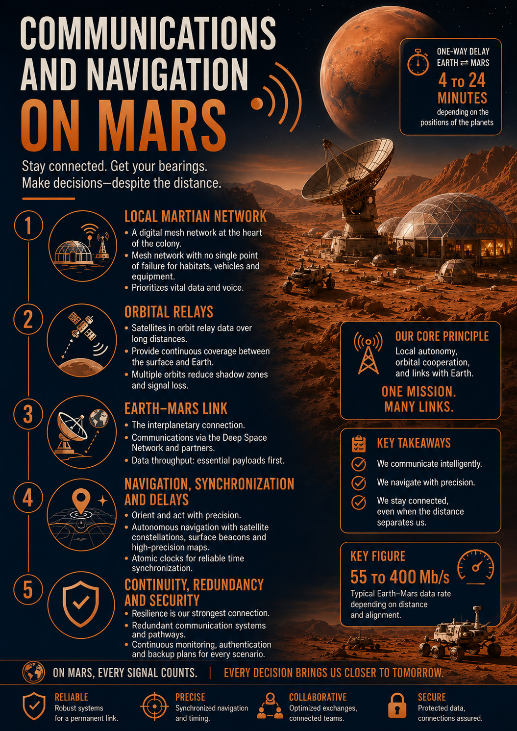
Interplanetary communications begins with a physical question: does the receiver collect enough signal energy to distinguish information from noise? It then becomes a network question: what happens when no path exists, which traffic is urgent and when does a command become stale? This module climbs from link budget to a disruption-tolerant Mars network.

1. Separate signal, physical link and service

Radio waves or laser beams carry modulated signals. Coding turns those signals into symbols and frames; protocols turn frames into network services. Failure can occur at any layer: insufficient power, lost pointing, corrupted frames, unavailable routes or stale applications. Troubleshooting starts by identifying which layer has actually failed.

Space communications can be described in layers. The physical signal carries symbols; the link turns symbols into frames through modulation, coding and synchronisation; the service decides which information has priority, what latency is acceptable and what happens when no end-to-end path exists. Mixing those layers creates poor reasoning: more transmitter power can improve a weak link without fixing a badly prioritised data queue, while a perfect protocol cannot compensate for an antenna pointed away from Earth. Engineers should be able to trace information from the sensor that creates it to the user who needs it and identify at which layer the margin or failure actually exists.

2. Use decibels to add gains and losses

For a power ratio P₂/P₁, decibel change is G = 10 log₁₀(P₂/P₁). A factor of ten is +10 dB; a factor of one hundred is +20 dB. Decibels let link engineers add gains and subtract losses instead of multiplying very large ratios.

Exercise A — simple conversion

An amplifier multiplies power by 100. What gain is that in dB?

G = 10 log₁₀(100) = 20 dB.

The decibel, dB, turns multiplicative ratios into additions. For a power ratio P₂/P₁, change is 10 log₁₀(P₂/P₁). Doubling power gives about +3 dB; multiplying by ten gives +10 dB; a −6 dB loss leaves roughly one quarter of the power. This is convenient for link budgets because gains and losses can be added, but the reference must be explicit. dBW is referenced to 1 watt while dBm is referenced to 1 milliwatt. Mixing dB, dBW and dBm without declaring the reference can create errors of orders of magnitude while still looking like clean arithmetic.

3. Distance creates free-space path loss

In the ideal far field, energy spreads over an area that grows with distance squared. Free-space loss can be represented by L = (4πd/λ)², where d is range and λ wavelength. In decibels, use 10 log₁₀(L). Doubling distance adds roughly 6 dB of loss.

Free-space path loss grows with both distance and frequency. In logarithmic form it contains terms proportional to 20 log₁₀(d) and 20 log₁₀(f), plus a constant set by the chosen units. Doubling distance adds about 6 dB of loss, meaning the received power is roughly four times lower with otherwise identical antennas. Earth–Mars links therefore change dramatically across planetary geometry. A mission cannot compute one budget at ‘Mars distance’; it needs cases spanning distance, occultation, solar angle, antenna mode and pointing error to identify the true limiting condition.

4. Antenna gain trades field of view for concentration

A directive antenna does not create energy; it concentrates it and increases receive sensitivity in chosen directions. Narrow beams demand accurate pointing. Deep-space communications is therefore coupled to attitude knowledge and control.

Antenna gain concentrates energy into a direction. For a dish, gain increases strongly with diameter D relative to wavelength λ. Greater gain therefore comes with a narrower beam and tighter pointing requirement, making GNC part of the communications budget. Mechanical consequences matter as well: mass, deployment, stiffness, thermal environment and keep-out zones. A smaller antenna can have poorer nominal performance but a wider beam that remains useful in degraded attitude control. Crewed spacecraft often benefit from several antenna classes or modes rather than one device optimised only for peak data rate.

5. Bandwidth, data rate and signal-to-noise ratio are coupled

Higher data rate usually requires more bandwidth, more received signal quality, more efficient coding or a combination. Mission throughput is lower than a laboratory peak because coding overhead, retransmissions, contact scheduling and outages consume capacity.

Exercise B — contact volume

A useful link delivers 8 Mbit/s for 25 minutes. What ideal volume is transferred?

25 min = 1,500 s. V = 8 × 1,500 = 12,000 Mbit = 1,500 MB, approximately 1.5 GB before overhead and interruptions.

Data rate is coupled to energy per bit. If received power remains constant while bit rate increases, less energy is available for each bit and decoding margin falls. E_b/N_0 compares energy per bit E_b with noise spectral density N_0. Error-correcting codes allow reliable communication at lower raw margin by adding structured redundancy and processing. A mission can therefore reduce data rate when distance grows or pointing degrades. Service design decides which information can wait and which justifies a more robust modulation, stronger code or greater energy expenditure. The radio and the operations schedule are consequently part of the same resource trade.

6. Radio and optical links solve different parts of the problem

Laser communications can deliver high data volume with narrow beams; radio offers mature acquisition and robust service across many phases. A hybrid architecture chooses by geometry, pointing, weather at Earth terminals, mission phase and criticality. Two media are not independent if the same power bus or pointing system can disable both.

Radio and optical links solve different problems rather than being absolute competitors. Optical communications can provide high data rates with very narrow beams, but require precise pointing and ground terminals that are affected by clouds and atmospheric conditions. Radio has extensive flight heritage, often more forgiving beamwidth and mature ground networks, but limited spectrum and potentially large antennas. A resilient architecture can use optical links for bulk transfer while retaining robust radio for command, safety or poor ground weather. Diversity only creates resilience if the two paths do not share all of their power, pointing, software and scheduling dependencies.

7. Latency is a physical boundary

Minimum propagation time is t = d/c, where d is distance and c the speed of light. Compression changes volume, not light-time. Mars operations therefore require asynchronous interaction and local authority.

Interplanetary latency is set by the speed of light. Earth and Mars range from tens to hundreds of millions of kilometres apart, so one-way light time is measured in minutes—roughly a few minutes to more than twenty depending on geometry. No network protocol can turn that into an instantaneous conversation. Operations must therefore decide what authority stays onboard, which questions can wait and which evidence should be transmitted before Earth asks for it. Latency is consequently an organisational and autonomy constraint as much as a radio property.

8. DTN stores information until a path exists

Delay/Disruption Tolerant Networking permits a node to hold a bundle when end-to-end connectivity is absent, then forward it later. This maps naturally to orbital relays, occultations and interplanetary gaps. Storage, expiration and integrity are network resources.

Delay/Disruption Tolerant Networking assumes that an end-to-end path may disappear. Instead of discarding data immediately, nodes store bundles and forward them when contact becomes available. Capacity planning must include memory, outage duration, priority and expiration rules. A camera producing 2 Mbit/s for six hours without a link creates 2 × 3,600 × 6 = 43,200 Mbit, about 5.4 GB before overhead. That simple calculation turns a network outage into a storage requirement. Recovery must also prevent old backlog from blocking urgent messages generated later.

9. Prioritise traffic by consequence and deadline

A few kilobytes of emergency telemetry may matter more than a huge science archive. Network policy needs service class, deadline, expiration, authenticity and confidentiality. An old command should be rejected even if its signature is valid.

A data queue should be prioritised by consequence and deadline, not only by file size. A safety command containing a few hundred bytes can be more important than a gigabyte of science. Categories can separate critical command, health telemetry, navigation, crew operations, science and deferrable transfers. Policy also defines what may be compressed, retransmitted or discarded. Priority without time can be misleading: weather information for an EVA planned two days from now is less urgent than a pressure alarm, yet useless if it arrives after the EVA. The network therefore carries operational intent as well as bits.

10. Failure scenario: primary relay disappears

Surface networking remains available, nonurgent data is queued, an alternate relay receives the highest-priority traffic and Earth gets a state summary at the next opportunity. The plan must also state queue capacity, expiration rules and the consequence of losing the backup relay.

Loss of a primary relay should be treated as a topology change. The spacecraft may fall back to a slower direct link, wait for another relay pass, alter attitude or reduce transmitted volume. Each option consumes something else: energy, time, GNC accuracy or storage. Operators need to know how long onboard memory can absorb data before saturation. Recovery includes validating the new route, replanning contacts and draining backlog in priority order. A resilient network does not promise that every link remains continuously available; it ensures that loss of one path does not destroy the life-critical service.

Guided case — six hours of communications blackout behind Mars

Assume a spacecraft produces an average 600 kbit/s of telemetry and useful data during a six-hour occultation. Raw volume is 600,000 × 21,600 ≈ 12.96 × 10⁹ bits, about 1.62 GB before coding, metadata and redundancy. If only 1 GB of queue storage is available, not everything can be retained. Operations must decide in advance which data is summarised, which rolling data may be overwritten and which critical records are protected from deletion.

When contact returns, sending 1.62 GB at 2 Mbit/s takes about 6,480 seconds, or 1.8 hours, if no new traffic is created. Real missions continue generating data, so recovery throughput must exceed average production or backlog never disappears. The difference between instantaneous link rate and queue balance is a fundamental network concept.

The case ends by losing the next relay as well. The service remains safe only if critical command has another path or local autonomy can wait. Network design is judged by continuity of function, not by permanent availability of every individual link.

11. Mini-project: close one communications service

Select EVA voice, habitat telemetry or science imagery.
Define useful data rate and acceptable delay.
Select RF, optical or hybrid transport.
List major gains and losses.
Add a 45-minute outage.
Define storage, priority and recovery behaviour.

The result is a usable service definition rather than merely a frequency and an antenna.

12. Mission lab — close a simplified link budget

Consider a teaching chain in decibels: transmit power +40 dBm, transmit antenna gain +30 dB, path loss −210 dB, receive antenna gain +65 dB, and miscellaneous loss −5 dB. Estimated received power is 40 + 30 − 210 + 65 − 5 = −80 dBm. dBm is power referenced to one milliwatt; dB is a ratio. The answer becomes meaningful only when compared with the receiver requirement for the selected modulation, coding and data rate.

If required sensitivity is −85 dBm, the example has 5 dB of raw margin. Real allocation then accounts for pointing, implementation loss, propagation effects, equipment variation and ageing. Every term should have an owner and source so a frequency or antenna change can be propagated through the budget rather than hidden in a generic margin.

Next test the same link in time. A superb eight-minute pass followed by fifty-two minutes with no path may be excellent for file delivery and unsuitable for a different operational service. Contact schedule, queue size and deadline are part of communications capacity.

A link budget also needs a noise model. Received power alone does not tell whether the receiver can decode. Thermal noise, bandwidth and receiver noise figure contribute to signal-to-noise metrics. The Academy keeps the first arithmetic simple, but the next engineering step is always to compare received signal against the correct noise and coding threshold.

13. From link to network: outage, storage and resumption

Assume an orbital relay is unavailable for 90 minutes while a habitat produces 2 Mbit/s of noncritical data. Required queue capacity is V = R × t = 2 × 5,400 = 10,800 Mbit, about 1.35 GB. This simple result shows that disruption tolerance consumes local storage as well as protocol logic. Redundancy, metadata and reserve increase the real allocation.

When contact returns, “first in, first out” may be wrong. A recent medical alert can outrank older science files. Stale commands may need to expire rather than execute. Network recovery therefore combines priority, age, authority and custody. DTN is most useful when these policies are explicit rather than treated as a magical store-and-forward feature.

Finally, rehearse loss of the alternate relay too. Which local services remain? How many hours of queue capacity exist? Which data can be discarded safely? Which navigation and timing functions are local? A communications architecture is resilient when those answers are known before the outage.

Calculation laboratory — formula reasoning

Space communications: quantitative mini-lessons

Signal-to-noise ratio in decibels

SNR_dB = 10 log10(P_signal / P_noise)

1 — Concrete question: What does “SNR_dB = 10 log10(P_signal / P_noise)” compute in the context of “Signal-to-noise ratio in decibels”?
2 — Intuition without symbols: Signal-to-noise ratio compares useful signal power with noise power, and the logarithmic scale converts it to decibels.
3 — Quantities: SNR_dB: ratio in dB; P_signal: signal power; P_noise: noise power.
4 — Formula: SNR_dB = 10 log10(P_signal / P_noise)
5 — Read aloud: Read “SNR_dB = 10 log10(P_signal / P_noise)” by naming every operation explicitly.
6 — Symbols and meaning: SNR_dB: ratio in dB; P_signal: signal power; P_noise: noise power.
7 — Pronunciation: The “Read aloud” line above is the oral reference for “Signal-to-noise ratio in decibels”. Any subscript, exponent or grouping that changes the meaning of the relation should be spoken explicitly.
8 — Units: Powers must use the same unit; their ratio is dimensionless; result in dB.
9 — Convention: For “Signal-to-noise ratio in decibels”, substitute values without changing the reference frame, time basis, system boundary or sign convention halfway through the calculation. Stated units: Powers must use the same unit; their ratio is dimensionless; result in dB.
10 — Why this operation: A power ratio converts to dB using 10 log10.
11 — Assumptions: Powers integrated over the same bandwidth and at the same chain point.
12 — Unit check: Powers must use the same unit; their ratio is dimensionless; result in dB. Verify that units reduce to the announced output quantity.
13 — Numerical case: If P_signal/P_noise = 100, SNR_dB = 10 log10(100) = 20 dB.
14 — Why the calculation works: A power ratio converts to dB using 10 log10.
15 — Algebraic check: 10^(SNR_dB/10) must recover linear ratio 100.
16 — Mental estimate: A ratio 100 = 10² corresponds exactly to 20 dB.
17 — Interpretation: Available SNR must be compared with the threshold required by modulation and coding.
18 — What the result does not prove: For “Signal-to-noise ratio in decibels”, the number obtained answers only the model “SNR_dB = 10 log10(P_signal / P_noise)” under the stated scenario. It does not by itself validate the input data or the model outside those conditions.
19 — Sensitivity: Multiplying power ratio by 10 adds 10 dB.
20 — Guided and autonomous exercises: Guided exercise. Linear ratio = 20.
Detailed guided correction — open after trying
SNR = 10 log10(20) = 13.01 dB.
Autonomous exercise. Linear ratio = 10.
Autonomous correction — open after trying
SNR = 10 log10(10) = 10.00 dB.
21 — Mission decision: Keep SNR margin above the link threshold, not merely equality at minimum.

Gain or loss from a power ratio

G_dB = 10 log10(P₂ / P₁)

1 — Concrete question: What does “G_dB = 10 log10(P₂ / P₁)” compute in the context of “Gain or loss from a power ratio”?
2 — Intuition without symbols: Decibels compress large power ratios into additions and subtractions that combine easily in a link budget.
3 — Quantities: G_dB: gain/loss in dB; P₂/P₁: power ratio.
4 — Formula: G_dB = 10 log10(P₂ / P₁)
5 — Read aloud: Read “G_dB = 10 log10(P₂ / P₁)” by naming every operation explicitly.
6 — Symbols and meaning: G_dB: gain/loss in dB; P₂/P₁: power ratio.
7 — Pronunciation: The “Read aloud” line above is the oral reference for “Gain or loss from a power ratio”. Any subscript, exponent or grouping that changes the meaning of the relation should be spoken explicitly.
8 — Units: P₂ and P₁ in the same unit; dimensionless ratio; result in dB.
9 — Convention: For “Gain or loss from a power ratio”, substitute values without changing the reference frame, time basis, system boundary or sign convention halfway through the calculation. Stated units: P₂ and P₁ in the same unit; dimensionless ratio; result in dB.
10 — Why this operation: The logarithmic definition turns power multiplications into dB additions.
11 — Assumptions: Positive ratio of comparable powers.
12 — Unit check: P₂ and P₁ in the same unit; dimensionless ratio; result in dB. Verify that units reduce to the announced output quantity.
13 — Numerical case: For P₂/P₁ = 100, G_dB = 10 log10(100) = 20 dB.
14 — Why the calculation works: The logarithmic definition turns power multiplications into dB additions.
15 — Algebraic check: 10^(20/10) = 100.
16 — Mental estimate: ×10 is +10 dB; ×100 is +20 dB.
17 — Interpretation: This relation lets gains and losses be added in the logarithmic domain.
18 — What the result does not prove: For “Gain or loss from a power ratio”, the number obtained answers only the model “G_dB = 10 log10(P₂ / P₁)” under the stated scenario. It does not by itself validate the input data or the model outside those conditions.
19 — Sensitivity: Halving power produces about −3.01 dB.
20 — Guided and autonomous exercises: Guided exercise. P₂/P₁ = 4.
Detailed guided correction — open after trying
G = 10 log10(4) = 6.02 dB.
Autonomous exercise. P₂/P₁ = 0.1.
Autonomous correction — open after trying
G = 10 log10(0.1) = −10.00 dB.
21 — Mission decision: Verify the sign of each term before summing a link budget.

Free-space path loss

L_FS,dB = 20 log10(4πd / λ)

1 — Concrete question: What does “L_FS,dB = 20 log10(4πd / λ)” compute in the context of “Free-space path loss”?
2 — Intuition without symbols: Power spreads geometrically with distance; wavelength also sets the electrical scale of propagation.
3 — Quantities: L_FS,dB: path loss in dB; d: distance; λ: wavelength.
4 — Formula: L_FS,dB = 20 log10(4πd / λ)
5 — Read aloud: Read “L_FS,dB = 20 log10(4πd / λ)” by naming every operation explicitly.
6 — Symbols and meaning: L_FS,dB: path loss in dB; d: distance; λ: wavelength.
7 — Pronunciation: The “Read aloud” line above is the oral reference for “Free-space path loss”. Any subscript, exponent or grouping that changes the meaning of the relation should be spoken explicitly.
8 — Units: d and λ in the same unit; result in dB.
9 — Convention: For “Free-space path loss”, substitute values without changing the reference frame, time basis, system boundary or sign convention halfway through the calculation. Stated units: d and λ in the same unit; result in dB.
10 — Why this operation: Linear loss is (4πd/λ)²; 10 log of the square becomes 20 log.
11 — Assumptions: Ideal free-space propagation without other losses.
12 — Unit check: d and λ in the same unit; result in dB. Verify that units reduce to the announced output quantity.
13 — Numerical case: With d = 1,000 km = 1×10⁶ m and λ = 0.10 m, L_FS ≈ 161.98 dB.
14 — Why the calculation works: Linear loss is (4πd/λ)²; 10 log of the square becomes 20 log.
15 — Algebraic check: Doubling d should add about 6.02 dB loss.
16 — Mental estimate: Very large distance quickly produces losses above one hundred decibels.
17 — Interpretation: Free-space loss is only one budget term; pointing, atmosphere and hardware can add others.
18 — What the result does not prove: For “Free-space path loss”, the number obtained answers only the model “L_FS,dB = 20 log10(4πd / λ)” under the stated scenario. It does not by itself validate the input data or the model outside those conditions.
19 — Sensitivity: L_FS rises by 6.02 dB when d doubles or λ halves.
20 — Guided and autonomous exercises: Guided exercise. d = 2,000 km, λ = 0.10 m.
Detailed guided correction — open after trying
L_FS = 20 log10(4π × 2×10⁶ / 0.10) ≈ 168.00 dB.
Autonomous exercise. d = 1,000 km, λ = 0.05 m.
Autonomous correction — open after trying
L_FS = 20 log10(4π × 1×10⁶ / 0.05) ≈ 168.00 dB.
21 — Mission decision: Include this loss in the budget before deciding on power, antennas or data rate.

Radio propagation time

t_prop = d / c

1 — Concrete question: What does “t_prop = d / c” compute in the context of “Radio propagation time”?
2 — Intuition without symbols: Even at light speed, interplanetary distance imposes an irreducible delay.
3 — Quantities: t_prop: one-way time; d: distance; c: speed of light.
4 — Formula: t_prop = d / c
5 — Read aloud: Read “t_prop = d / c” by naming every operation explicitly.
6 — Symbols and meaning: t_prop: one-way time; d: distance; c: speed of light.
7 — Pronunciation: The “Read aloud” line above is the oral reference for “Radio propagation time”. Any subscript, exponent or grouping that changes the meaning of the relation should be spoken explicitly.
8 — Units: t in s; d in m; c = 299,792,458 m/s.
9 — Convention: For “Radio propagation time”, substitute values without changing the reference frame, time basis, system boundary or sign convention halfway through the calculation. Stated units: t in s; d in m; c = 299,792,458 m/s.
10 — Why this operation: Time is distance divided by propagation speed.
11 — Assumptions: Geometric path distance and electromagnetic propagation in vacuum.
12 — Unit check: t in s; d in m; c = 299,792,458 m/s. Verify that units reduce to the announced output quantity.
13 — Numerical case: For d = 225×10⁹ m, t_prop ≈ 225×10⁹/299,792,458 = 750.5 s = 12.51 min.
14 — Why the calculation works: Time is distance divided by propagation speed.
15 — Algebraic check: c·t must recover about 225 billion metres.
16 — Mental estimate: 300,000 km/s for 750 s is about 225 million km.
17 — Interpretation: This delay prevents instantaneous conversational control of Mars operations.
18 — What the result does not prove: For “Radio propagation time”, the number obtained answers only the model “t_prop = d / c” under the stated scenario. It does not by itself validate the input data or the model outside those conditions.
19 — Sensitivity: Propagation time varies linearly with distance.
20 — Guided and autonomous exercises: Guided exercise. d = 150×10⁹ m.
Detailed guided correction — open after trying
t ≈ 500.35 s = 8.34 min.
Autonomous exercise. d = 75×10⁹ m.
Autonomous correction — open after trying
t ≈ 250.17 s = 4.17 min.
21 — Mission decision: Design procedures and local autonomy using actual round-trip delay.

Data volume generated or transmitted

V = R × t

1 — Concrete question: What does “V = R × t” compute in the context of “Data volume generated or transmitted”?
2 — Intuition without symbols: A data rate becomes total data volume when multiplied by the time over which it applies.
3 — Quantities: V: data volume; R: data rate; t: duration.
4 — Formula: V = R × t
5 — Read aloud: Read “V = R × t” by naming every operation explicitly.
6 — Symbols and meaning: V: data volume; R: data rate; t: duration.
7 — Pronunciation: The “Read aloud” line above is the oral reference for “Data volume generated or transmitted”. Any subscript, exponent or grouping that changes the meaning of the relation should be spoken explicitly.
8 — Units: R in bit/s or Mbit/s; t in s; V in corresponding bits.
9 — Convention: For “Data volume generated or transmitted”, substitute values without changing the reference frame, time basis, system boundary or sign convention halfway through the calculation. Stated units: R in bit/s or Mbit/s; t in s; V in corresponding bits.
10 — Why this operation: Rate is quantity per second; multiplication by time accumulates total quantity.
11 — Assumptions: Representative average rate over the interval.
12 — Unit check: R in bit/s or Mbit/s; t in s; V in corresponding bits. Verify that units reduce to the announced output quantity.
13 — Numerical case: At 8 Mbit/s for 1,500 s, V = 8×1,500 = 12,000 Mbit = 1,500 MB ≈ 1.5 GB before overhead.
14 — Why the calculation works: Rate is quantity per second; multiplication by time accumulates total quantity.
15 — Algebraic check: V/t must recover 8 Mbit/s and 8 bits = 1 byte.
16 — Mental estimate: 8 Mbit/s for 25 min gives about 12 Gbit, or 1.5 GB.
17 — Interpretation: Raw volume must then account for protocol, coding, retransmission and margin.
18 — What the result does not prove: For “Data volume generated or transmitted”, the number obtained answers only the model “V = R × t” under the stated scenario. It does not by itself validate the input data or the model outside those conditions.
19 — Sensitivity: V varies linearly with rate and duration.
20 — Guided and autonomous exercises: Guided exercise. R = 2 Mbit/s for 5,400 s.
Detailed guided correction — open after trying
V = 10,800 Mbit = 1,350 MB ≈ 1.35 GB.
Autonomous exercise. R = 40 Mbit/s over two 1,500 s windows.
Autonomous correction — open after trying
V = 40×3,000 = 120,000 Mbit = 15,000 MB ≈ 15 GB.
21 — Mission decision: Size storage and communication schedule using actual net transferable volume.

Received-power link budget

P_r,dBm = P_t,dBm + G_t + G_r − L_path − L_misc

1 — Concrete question: What does “P_r,dBm = P_t,dBm + G_t + G_r − L_path − L_misc” compute in the context of “Received-power link budget”?
2 — Intuition without symbols: In the decibel domain, gains and losses add algebraically to give received power.
3 — Quantities: P_r: received power; P_t: transmitted power; G_t/G_r: antenna gains; L_path: path loss; L_misc: additional losses.
4 — Formula: P_r,dBm = P_t,dBm + G_t + G_r − L_path − L_misc
5 — Read aloud: Read “P_r,dBm = P_t,dBm + G_t + G_r − L_path − L_misc” by naming every operation explicitly.
6 — Symbols and meaning: P_r: received power; P_t: transmitted power; G_t/G_r: antenna gains; L_path: path loss; L_misc: additional losses.
7 — Pronunciation: The “Read aloud” line above is the oral reference for “Received-power link budget”. Any subscript, exponent or grouping that changes the meaning of the relation should be spoken explicitly.
8 — Units: P_t and P_r in dBm; gains/losses in dB.
9 — Convention: For “Received-power link budget”, substitute values without changing the reference frame, time basis, system boundary or sign convention halfway through the calculation. Stated units: P_t and P_r in dBm; gains/losses in dB.
10 — Why this operation: Multiplicative ratios become dB sums; losses enter with negative sign.
11 — Assumptions: All terms refer to the same link scenario and frequency.
12 — Unit check: P_t and P_r in dBm; gains/losses in dB. Verify that units reduce to the announced output quantity.
13 — Numerical case: With P_t = 40 dBm, G_t = 30 dB, G_r = 65 dB, L_path = 210 dB and L_misc = 5 dB, P_r = −80 dBm.
14 — Why the calculation works: Multiplicative ratios become dB sums; losses enter with negative sign.
15 — Algebraic check: Re-adding gains and losses must reconstruct the chain without sign errors.
16 — Mental estimate: 40+30+65 = 135; 210+5 = 215; 135−215 = −80 dBm.
17 — Interpretation: Received power must then be compared with noise and receiver sensitivity.
18 — What the result does not prove: For “Received-power link budget”, the number obtained answers only the model “P_r,dBm = P_t,dBm + G_t + G_r − L_path − L_misc” under the stated scenario. It does not by itself validate the input data or the model outside those conditions.
19 — Sensitivity: Each additional dB of loss lowers P_r by one dB.
20 — Guided and autonomous exercises: Guided exercise. 43 + 32 + 60 − 205 − 4.
Detailed guided correction — open after trying
P_r = 135−209 = −74 dBm.
Autonomous exercise. 38 + 28 + 62 − 208 − 6.
Autonomous correction — open after trying
P_r = 128−214 = −86 dBm.
21 — Mission decision: Validate data rate only after closing both power and SNR budgets.

Radio-photon energy

E_photon = h f

1 — Concrete question: What does “E_photon = h f” compute in the context of “Radio-photon energy”?
2 — Intuition without symbols: At higher frequency, each electromagnetic quantum carries more energy, even though radio links are usually treated in collective power and noise terms.
3 — Quantities: E_photon: energy; h: Planck constant; f: frequency.
4 — Formula: E_photon = h f
5 — Read aloud: Read “E_photon = h f” by naming every operation explicitly.
6 — Symbols and meaning: E_photon: energy; h: Planck constant; f: frequency.
7 — Pronunciation: The “Read aloud” line above is the oral reference for “Radio-photon energy”. Any subscript, exponent or grouping that changes the meaning of the relation should be spoken explicitly.
8 — Units: E in J; h = 6.62607015×10⁻³⁴ J·s; f in Hz.
9 — Convention: For “Radio-photon energy”, substitute values without changing the reference frame, time basis, system boundary or sign convention halfway through the calculation. Stated units: E in J; h = 6.62607015×10⁻³⁴ J·s; f in Hz.
10 — Why this operation: Planck relation directly links frequency and quantum energy.
11 — Assumptions: Well-defined frequency; quantum interpretation without confusing single-photon energy with total signal power.
12 — Unit check: E in J; h = 6.62607015×10⁻³⁴ J·s; f in Hz. Verify that units reduce to the announced output quantity.
13 — Numerical case: At f = 8.4 GHz, E = 6.626×10⁻³⁴×8.4×10⁹ ≈ 5.57×10⁻²⁴ J.
14 — Why the calculation works: Planck relation directly links frequency and quantum energy.
15 — Algebraic check: E/f must recover h.
16 — Mental estimate: Doubling frequency doubles photon energy.
17 — Interpretation: This scale links wave, thermal-noise and quantum descriptions, but does not size the link alone.
18 — What the result does not prove: For “Radio-photon energy”, the number obtained answers only the model “E_photon = h f” under the stated scenario. It does not by itself validate the input data or the model outside those conditions.
19 — Sensitivity: E_photon varies linearly with f.
20 — Guided and autonomous exercises: Guided exercise. f = 2.2 GHz.
Detailed guided correction — open after trying
E ≈ 6.626×10⁻³⁴×2.2×10⁹ = 1.46×10⁻²⁴ J.
Autonomous exercise. f = 32 GHz.
Autonomous correction — open after trying
E ≈ 2.12×10⁻²³ J.
21 — Mission decision: Keep this relation as physical insight; size the link with power, noise, antennas and coding.

Mission reasoning lab — reason about a Mars communication link

Scenario. At the receiver, useful signal power is 100 times the noise power in the defined bandwidth. The linear signal-to-noise ratio is therefore 100 and SNR = 10 log10(100) = 20 dB. If signal power falls by a factor of ten while noise stays fixed, SNR becomes 10 dB. These simple anchors should be known before using a full link-budget spreadsheet.

1. Keep power ratios and amplitude ratios distinct

The 10·log10 rule applies to power ratios. A 20·log10 coefficient is used for appropriate amplitude ratios when power is proportional to amplitude squared. Confusing the two creates a factor-of-two error in decibels that can completely overturn a link-margin conclusion.

2. Bandwidth belongs in every noise statement

Noise power generally increases with receiver bandwidth. Quoting a noise figure or SNR without defining bandwidth can therefore be misleading. A narrowband carrier and a high-data-rate channel can experience very different noise totals even at the same antenna and temperature.

3. Distance creates severe free-space loss

Earth–Mars range changes dramatically over the synodic cycle. Received power from an ideal free-space link falls approximately with the square of distance. Doubling range costs about 6 dB of free-space path loss. A communication design that works only at favourable geometry is not an all-mission design.

4. Antenna gain trades against pointing

A larger, more directive antenna can recover link margin, but its beam becomes narrower and pointing requirements become tighter. The apparent “free gain” therefore moves difficulty into attitude knowledge, mechanical stability and operations. High gain does not create energy; it concentrates it spatially.

5. Light-time changes operations

Even with a perfect radio link, Mars cannot be teleoperated from Earth like a nearby drone. One-way light time ranges from minutes to more than twenty minutes depending on geometry. Commanding, fault response and scientific operations therefore require onboard autonomy, store-and-forward networking and procedures that tolerate delay.

6. Inverse problem — required power ratio

If a modem requires 13 dB SNR under the chosen coding and bandwidth, the equivalent linear power ratio is 10^(13/10) ≈ 20. If the current ratio is only 10, the system needs roughly a factor of two improvement in signal-to-noise power ratio. That improvement might come from transmitter power, antenna gain, lower loss, narrower bandwidth, lower receiver noise or different coding; the equation does not dictate which architecture is best.

Decision check

A credible link statement should name transmitter power, antenna gains, frequency, distance, propagation losses, receiver noise assumptions, bandwidth, coding/modulation requirement and margin. If SNR is quoted without those conditions, treat it as a partial result rather than proof that communication will work.

Link resilience and operations

Solar conjunction. When the Sun lies near the Earth–Mars line of sight, plasma and geometry can degrade communications. Mission plans reduce command activity, increase autonomy and tolerate data backlog. A link budget that ignores conjunction cannot represent full-mission availability.

Store-and-forward networking. Deep-space communication is intermittent. Delay-tolerant networking stores data until a path becomes available and forwards it later. This changes the operational question from “is there a continuous connection?” to “can critical information survive disruption and arrive before its deadline?”

Priority classes. Emergency commands, health telemetry, engineering logs and bulk science data do not have the same urgency. Bandwidth allocation should preserve command and safety channels under degraded conditions before maximizing science throughput.

Pointing loss. A high-gain antenna can lose many decibels if pointing error moves the target away from the beam centre. Link analysis therefore includes pointing knowledge, control error and structural distortion. The antenna pattern and attitude-control system are part of the same communication architecture.

Verification. End-to-end tests should include realistic delays, outages, corrupted packets, clock errors and failover paths. A modem that works perfectly on a bench cable has not yet demonstrated a Mars communication service.

Final communication check

Availability must be evaluated over time, not from one favourable geometry. Track daily and seasonal variations in range, antenna visibility, relay coverage, maintenance outages and conjunction periods. The resulting service availability is often more operationally meaningful than a single peak data rate.

Security also belongs in the link architecture. Authentication, key management, replay protection and command authorization must remain functional despite long delay and intermittent contact. A Mars communication system that delivers bits reliably but cannot establish trustworthy command provenance is not mission-ready.

Zero-prerequisite concepts

photon

Definition. A photon is a quantum of electromagnetic radiation. Radio communication can be described at the electromagnetic-wave level while photon energy is linked to frequency by E = hf.

Example. A radio transmitter launches electromagnetic energy that propagates at the speed of light in vacuum.

Pitfall. Photon language does not replace practical link quantities such as power, bandwidth, noise and antenna gain.

Higher photon frequency means higher photon energy and shorter wavelength in vacuum.

Guided exercise — photon

Situation to recognize. A photon is a quantum of electromagnetic radiation. Radio communication can be described at the electromagnetic-wave level while photon energy is linked to frequency by E = hf.

Check requested. Higher photon frequency means higher photon energy and shorter wavelength in vacuum.

Error to reject. Photon language does not replace practical link quantities such as power, bandwidth, noise and antenna gain.

Reasoned solution

Precise meaning: A photon is a quantum of electromagnetic radiation. Radio communication can be described at the electromagnetic-wave level while photon energy is linked to frequency by E = hf.
Case test: Higher photon frequency means higher photon energy and shorter wavelength in vacuum.
Excluded pitfall: Photon language does not replace practical link quantities such as power, bandwidth, noise and antenna gain.
Operational consequence: Use this check before accepting a result in mission design: Higher photon frequency means higher photon energy and shorter wavelength in vacuum.

Quantification: photon: use the unit or dimension defined by the physical quantity; if the concept is qualitative, do not invent a numerical unit.
Verification: photon: compare the conclusion with the mental check and the stated pitfall.

frequency

Definition. Frequency is the number of oscillation cycles per second, measured in hertz (Hz).

Example. X-band and Ka-band links use different frequency ranges and therefore different antenna and propagation trade-offs.

Pitfall. A higher carrier frequency does not automatically mean a higher end-to-end data rate.

Frequency and period are inverses: doubling frequency halves period.

Guided exercise — frequency

Situation to recognize. Frequency is the number of oscillation cycles per second, measured in hertz (Hz).

Check requested. Frequency and period are inverses: doubling frequency halves period.

Error to reject. A higher carrier frequency does not automatically mean a higher end-to-end data rate.

Reasoned solution

Precise meaning: Frequency is the number of oscillation cycles per second, measured in hertz (Hz).
Case test: Frequency and period are inverses: doubling frequency halves period.
Excluded pitfall: A higher carrier frequency does not automatically mean a higher end-to-end data rate.
Operational consequence: Use this check before accepting a result in mission design: Frequency and period are inverses: doubling frequency halves period.

Quantification: frequency: use the unit or dimension defined by the physical quantity; if the concept is qualitative, do not invent a numerical unit.
Verification: frequency: compare the conclusion with the mental check and the stated pitfall.

antenna gain

Definition. Antenna gain describes how strongly an antenna concentrates transmitted or received power in a direction relative to a reference.

Example. A large dish can provide high gain but requires more accurate pointing.

Pitfall. Gain does not create energy; it redistributes directivity.

A more directive antenna should have a narrower useful beam, all else equal.

Guided exercise — antenna gain

Situation to recognize. Antenna gain describes how strongly an antenna concentrates transmitted or received power in a direction relative to a reference.

Check requested. A more directive antenna should have a narrower useful beam, all else equal.

Error to reject. Gain does not create energy; it redistributes directivity.

Reasoned solution

Precise meaning: Antenna gain describes how strongly an antenna concentrates transmitted or received power in a direction relative to a reference.
Case test: A more directive antenna should have a narrower useful beam, all else equal.
Excluded pitfall: Gain does not create energy; it redistributes directivity.
Operational consequence: Use this check before accepting a result in mission design: A more directive antenna should have a narrower useful beam, all else equal.

Quantification: antenna gain: use the unit or dimension defined by the physical quantity; if the concept is qualitative, do not invent a numerical unit.
Verification: antenna gain: compare the conclusion with the mental check and the stated pitfall.

signal-to-noise ratio

Definition. Signal-to-noise ratio compares useful signal power with noise power at a defined point and bandwidth.

Example. A decoder needs adequate SNR for the chosen modulation and coding.

Pitfall. SNR must always be tied to bandwidth and measurement conditions.

If signal power rises while noise is unchanged, SNR must improve.

Guided exercise — signal-to-noise ratio

Situation to recognize. Signal-to-noise ratio compares useful signal power with noise power at a defined point and bandwidth.

Check requested. If signal power rises while noise is unchanged, SNR must improve.

Error to reject. SNR must always be tied to bandwidth and measurement conditions.

Reasoned solution

Precise meaning: Signal-to-noise ratio compares useful signal power with noise power at a defined point and bandwidth.
Case test: If signal power rises while noise is unchanged, SNR must improve.
Excluded pitfall: SNR must always be tied to bandwidth and measurement conditions.
Operational consequence: Use this check before accepting a result in mission design: If signal power rises while noise is unchanged, SNR must improve.

Quantification: signal-to-noise ratio: use the unit or dimension defined by the physical quantity; if the concept is qualitative, do not invent a numerical unit.
Verification: signal-to-noise ratio: compare the conclusion with the mental check and the stated pitfall.

Beginner vocabulary checkpoint

carrier signal — Radio-frequency waveform used to transport information across a communications link.
noise power — Unwanted received power that competes with the desired signal in a measurement bandwidth.
signal-to-noise ratio — Ratio between useful signal power and noise power, often expressed in decibels.
decibel — Logarithmic unit used for power ratios; 10 dB corresponds to a tenfold power ratio.
bandwidth — Frequency range occupied or processed by a communications channel.
data rate — Amount of information transmitted per unit time, commonly in bits per second.
modulation — Method used to encode information by varying a carrier waveform.
coding — Added structured redundancy that allows a receiver to detect or correct data errors.
antenna gain — Directional concentration of radiated or received power relative to a reference antenna.
EIRP — Equivalent isotropically radiated power combining transmitter power and transmitting antenna gain.
free-space path loss — Reduction in received power caused by geometric spreading with distance and wavelength.
link budget — Accounting of gains and losses from transmitter through propagation to receiver.
received power — Signal power delivered at the receiver input after propagation and antenna effects.
Doppler shift — Frequency change caused by relative motion between transmitter and receiver.
latency — Delay between sending information and receiving or acting on it.
one-way light time — Minimum propagation delay set by distance divided by the speed of light.
Deep Space Network — NASA network of large antennas used to communicate with distant spacecraft.
pointing loss — Link loss caused when antenna boresight is not perfectly aligned with the other terminal.

Sources and references

Verified primary supplement: NASA — Deep Space Network

Engineering studio — manage a data backlog

A mission generates 120 GB of data per day. Two 25-minute communication windows at 40 Mbit/s ideally carry 40×10⁶×(2×1,500) = 1.2×10¹¹ bits, or about 15 GB before protocol overhead and losses. The system therefore creates roughly 105 GB of data backlog per day. Units must remain consistent: 1 byte = 8 bits, and a bit/s data rate must be multiplied by time in seconds.

The workshop designs a queue policy: safety telemetry, irreplaceable science, compressible products and regenerable data do not deserve the same priority. One entire pass is then lost. The student computes backlog growth, defines the threshold for stronger compression or product deletion, and explains why onboard autonomy is required when latency prevents Earth from managing every packet in real time.

The communications capstone adds one more constraint: storage is finite. If backlog grows faster than contact capacity, the mission eventually reaches a point where prioritisation alone cannot prevent data loss. The student estimates the time to fill the available store, then defines which products are compressed, delayed or discarded first while keeping commanding, health telemetry and time-critical science protected.