AM-01.11 — Derivative: rate of change

Course compass

Question directrice : What is a derivative, how do we read f prime of x and dx/dt, and how does average slope become instantaneous change?

Free learning resource: this content is not professional training, a diploma, certification or professional authorization. Examples are educational and do not replace engineering, testing or qualification of real space hardware.

1 — The derivative starts with a speedometer question: “how fast is it changing now?”

A rover covers 100 m in 20 s, giving an average speed of 5 m/s. That does not say whether it was moving at 2 m/s first and 8 m/s later.

A derivative asks a more local question: how fast is a quantity changing at this instant?

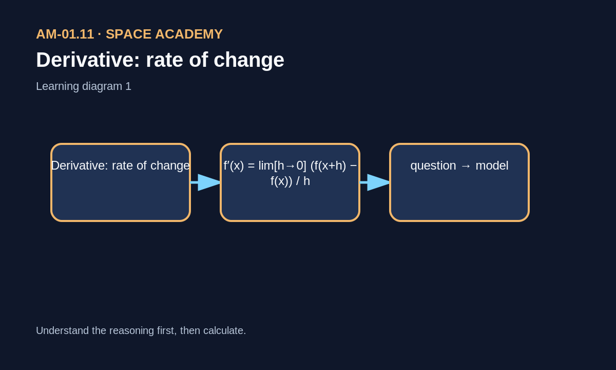
Average and instantaneous speed — A derivative looks for local change, not only the average over the whole trip.

2 — How do we read f′(x) and dx/dt?

f′(x) is read “f prime of x”. The prime mark indicates the derivative.

dx/dt is read “d x over d t” or “the derivative of x with respect to time t”. If x is metres and t seconds, dx/dt has units m/s.

3 — From average slope to local slope

average velocity = Δx ÷ Δt

To estimate velocity at one instant, choose measurements closer and closer around that instant. Average slope then approaches local slope.

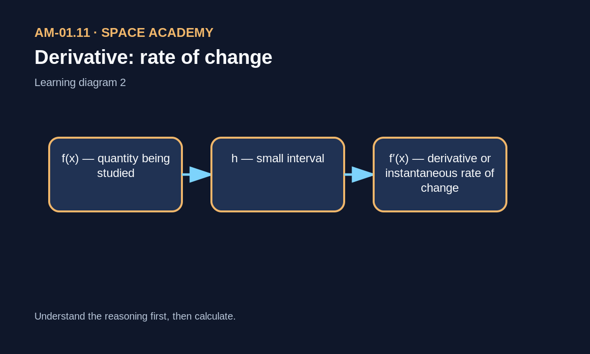
A derivative is not division by zero. We study what happens as the interval becomes very small; we do not simply put zero in the denominator.

Secant approaching tangent — Closer points make the average slope approach the local slope.

4 — Complete example 1: x(t)=2t²

x(t)=2t² is read “x of t equals two t squared”. Its derivative is dx/dt=4t.

At t=3 s: v=4×3=12 m/s. Around the third second, position increases at 12 metres per second in this model.

Rover position and velocity — The slope of position versus time gives instantaneous velocity.

5 — Complete example 2: falling tank pressure

Pressure falls from 300 kPa to 294 kPa between t=10 s and t=12 s.

ΔP = 294 − 300 = −6 kPa
Δt = 2 s
average rate = −6 ÷ 2 = −3 kPa/s

The negative sign means pressure is decreasing.

6 — Complete example 3: power ramp

Electrical power rises from 2 kW to 5 kW in 6 s.

ΔP = 3 kW
Δt = 6 s
average rate = 0.5 kW/s

An instantaneous derivative would reveal whether the ramp is smooth or includes a spike.

7 — Units explain the derivative

Position m / time s → velocity m/s. Velocity m/s / time s → acceleration m/s². Pressure kPa / time s → kPa/s.

Derivative units — Units reveal what physical rate is being measured.

8 — Real measurements: derivatives can amplify noise

Small sensor fluctuations can produce large apparent differences when two very close samples are subtracted. Engineers therefore filter signals and choose time intervals carefully.

9 — Numerical estimate from two nearby measurements

If x=48.2 m at 9.9 s and x=50.6 m at 10.1 s:

Δx=2.4 m
Δt=0.2 s
v≈2.4÷0.2=12 m/s

This estimates velocity around 10 s.

Numerical derivative estimate — Nearby samples estimate a local rate if sensor noise is controlled.

10 — What to remember

A derivative measures a local rate of change.
f′(x) is “f prime of x”.
dx/dt is “d x over d t”.
It extends average slope to a very small interval.
Its units are quantity-units divided by variable-units.
Real data require attention to noise and sampling.

Exercises and answers

Exercise 1

Position changes from 10 m to 16 m between 2 s and 4 s. Average velocity?

(16−10)/(4−2)=3 m/s.

Exercise 2

If x(t)=3t², derivative and value at t=2?

dx/dt=6t; at 2 s: 12 m/s if x is metres.

Exercise 3

Pressure falls 8 kPa in 4 s. Sign and rate?

Negative: −2 kPa/s.

AM-01.11 — Derivative: measuring how fast a quantity changes now