Engine controller: from sensor to decision

1 — The physical question

How does a controller turn a pressure or thrust error into a valve command?

We start from the concrete problem before notation. The goal is to understand what we seek, then why mathematics becomes useful.

2 — How to read the symbols and units

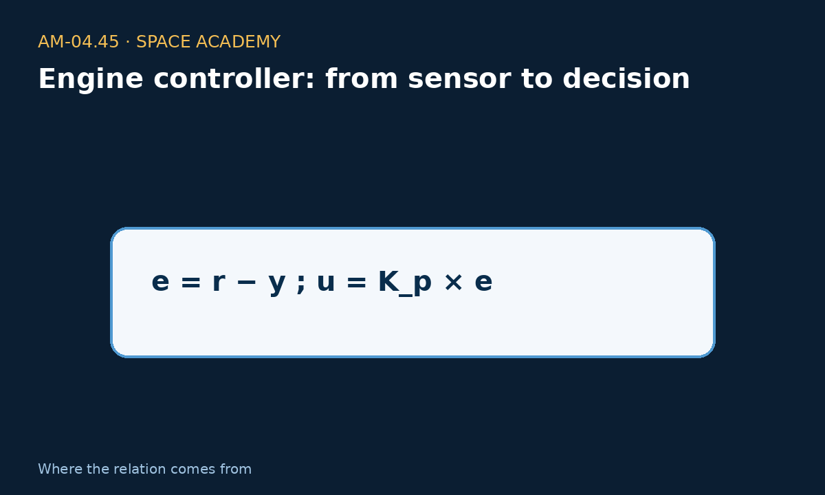
e = r − y ; u = K_p × e. Read: “e equals r minus y; u equals K p times e”.

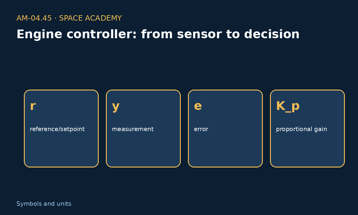
r — reference/setpoint ; y — measurement ; e — error ; K_p — proportional gain ; u — computed command

3 — Where does the relation come from?

A feedback loop compares reference r with measurement y. Error e feeds a control law. In the simplest proportional model, command u is Kp times error. Real controllers add filters, limits, state logic and protections.

Every number used below is explicitly treated as data, convention, learning assumption, or calculated result.

4 — A — Pressure too low

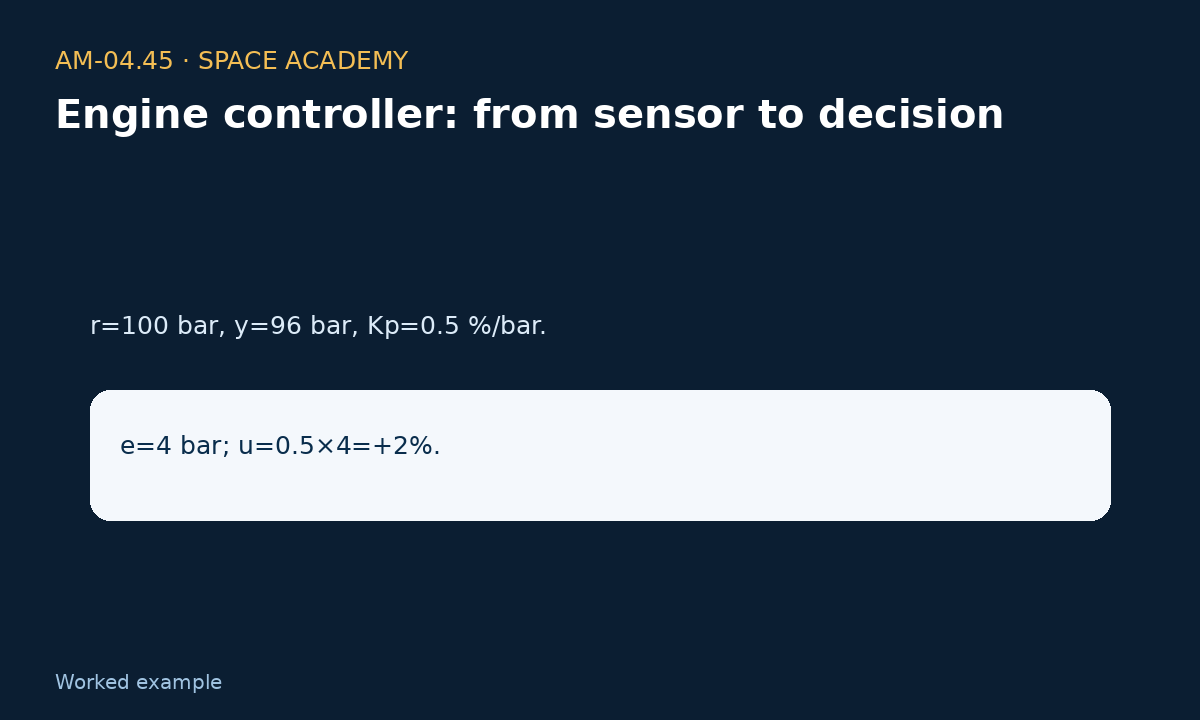
Where do the numbers come from? r=100 bar, y=96 bar, Kp=0.5 %/bar.

Step-by-step calculation: e=4 bar; u=0.5×4=+2%.

The model asks for a small command increase.

5 — B — Pressure too high

Where do the numbers come from? r=100, y=104, Kp=0.5.

Step-by-step calculation: e=−4; u=−2%.

The sign naturally reverses correction direction.

6 — C — Saturation

Where do the numbers come from? e=30 bar, Kp=0.5 => u=15%, but actuator limit is +8%.

Step-by-step calculation: Applied command = +8%, not +15%.

Physical limits must be built into logic; the equation alone can command the impossible.

7 — Sensitivity, inverse calculation, and sanity check

Change one input, predict the direction of the result, calculate, then check units, sign, order of magnitude, and limits.

Essential limit for Engine controller: from sensor to decision: the displayed relation is a learning model. A real system adds detailed geometry, variable properties, sensors, uncertainty, transients, and testing.

8 — Why this matters in a mission

In a space mission, how does a controller turn a pressure or thrust error into a valve command? The useful skill is not reciting the formula but knowing which data are needed, which are measured, and when the model becomes insufficient.

10 — Go deeper: from calculation to physical understanding

The loop begins with the difference between what we want and what we measure

In e=r-y, r is the command and y is the measured value. If commanded pressure is 100 units and measurement is 92, the error is +8. The sign tells the corrective direction under the chosen convention. This subtraction is at the heart of many control loops: act on error rather than blindly commanding a fixed actuator position.

Gain Kp turns error into action

In the learning model u=Kp e, a larger gain produces a stronger correction for the same error. That may seem always desirable, but a real loop contains delay, inertia, noise, and actuator limits. Excessive gain can produce overshoot or oscillation. Control is therefore a dynamics problem, not merely a multiplication.

Saturation reminds us that the machine has limits

If the calculation requests u=120% while the actuator can provide only 100%, the real command saturates at its limit. Software must know this: continuing to calculate as if 120% were actually applied can degrade loop behaviour. Even a beginner lesson should teach that a control equation always meets physical limits.

Automation does not remove the need for evidence

A computer can execute thousands of corrections per second, but speed does not prove that the logic is correct. Control laws, sensors, actuators, software, and degraded modes must be verified together. This principle explains how a modern launch vehicle can automatically correct attitude without a human “flying the nozzle” at every instant.

9 — Exercises and answers